

natural varying electromagnetic field as source. On land
the method (MT) was introduced in the 1950s by the
geophysicists Cagniard and Thikonov. MT can improve
the interpretation of deep structures as it has very low
frequency content, and it can image conductive
sediments below thick resistors such as salt or basalt.
For this reason the MMT application has created interest also in the hydrocarbon exploration industry.
20.2 CSEM Basic Concepts
20.2.1 Background
Resistivity variations in rocks are generally controlled
by the interplay between highly resistive minerals and
pore fluids including low resistive saline water and/or
highly resistive hydrocarbons. Sedimentary rocks
have a wide range of resistivities (0.2–1,000 Ωm)
mainly controlled by variations in porosity, permeability and pore connectivity geometries in addition to
pore fluid properties and temperature. It is the high
resistivity of hydrocarbon filled reservoir rocks
(30–500 Ωm) compared with reservoirs filled with
saline formation water (0.5–2 Ωm) that makes EM
sounding a good tool for detection of subsurface HC.
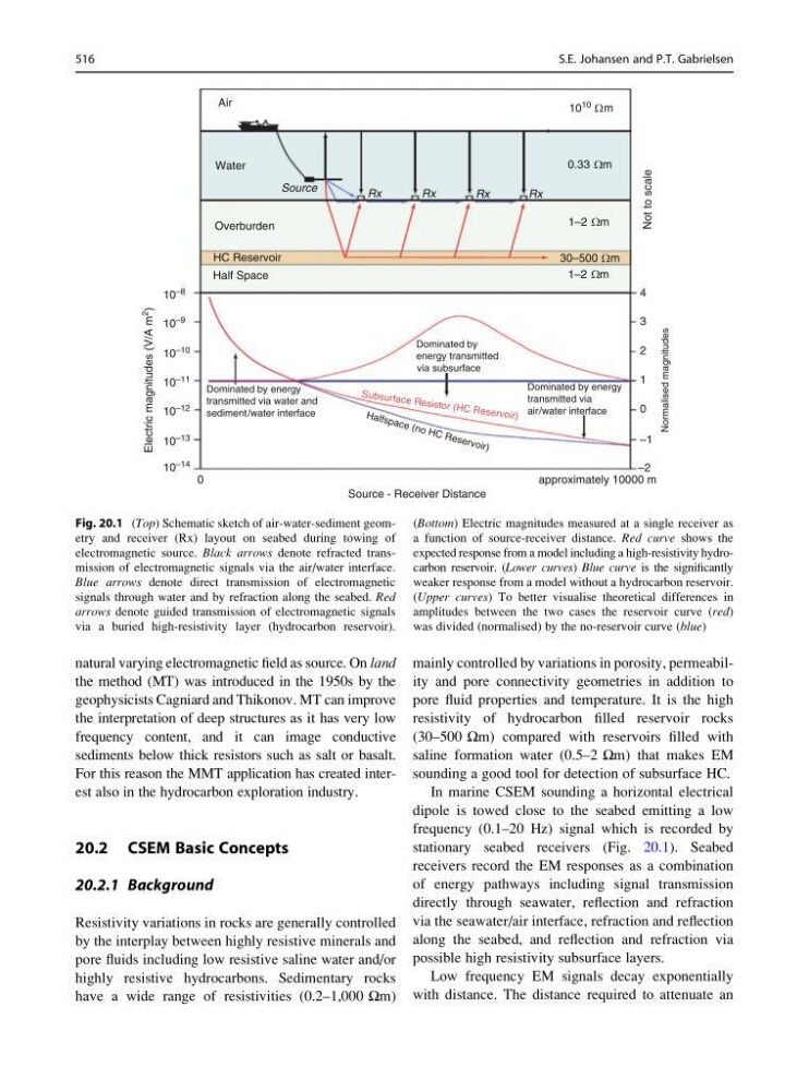
In marine CSEM sounding a horizontal electrical
dipole is towed close to the seabed emitting a low
frequency (0.1–20 Hz) signal which is recorded by
stationary seabed receivers (Fig. 20.1). Seabed
receivers record the EM responses as a combination
of energy pathways including signal transmission
directly through seawater, reflection and refraction
via the seawater/air interface, refraction and reflection
along the seabed, and reflection and refraction via
possible high resistivity subsurface layers.
Low frequency EM signals decay exponentially
with distance. The distance required to attenuate an
Air
Water
Source
Rx
Rx
Rx
Rx
0.33 m
Ω
10
10 m
Ω
30–500 m
Ω
1–2 m
Ω
1–2 m
Ω
4
3
2
1
0
–1
–2
approximately 10000 m
Overburden
Half Space
HC Reservoir
Dominated by energy
transmitted via water and
sediment/water interface
Dominated by energy
transmitted via
air/water interface
Dominated by
energy transmitted
via subsurface
Normalised magnitudes
Not to scale
Su bsu rfa ce Re sis tor (HC Re ser voi r)
H al fs pa ce (n o H C R es er vo ir)
10 –8
10 –11
10 –12
10 –13
10 –14
10 –10
10 –9
0
Source - Receiver Distance
Electric magnitudes (V/A m
2
)
Fig. 20.1 (Top) Schematic sketch of air-water-sediment geometry and receiver (Rx) layout on seabed during towing of
electromagnetic source. Black arrows denote refracted transmission of electromagnetic signals via the air/water interface.
Blue arrows denote direct transmission of electromagnetic
signals through water and by refraction along the seabed. Red
arrows denote guided transmission of electromagnetic signals
via a buried high-resistivity layer (hydrocarbon reservoir).
(Bottom) Electric magnitudes measured at a single receiver as
a function of source-receiver distance. Red curve shows the
expected response from a model including a high-resistivity hydrocarbon reservoir. (Lower curves) Blue curve is the significantly
weaker response from a model without a hydrocarbon reservoir.
(Upper curves) To better visualise theoretical differences in
amplitudes between the two cases the reservoir curve (red)
was divided (normalised) by the no-reservoir curve (blue)
516
S.E. Johansen and P.T. Gabrielsen
the method (MT) was introduced in the 1950s by the
geophysicists Cagniard and Thikonov. MT can improve
the interpretation of deep structures as it has very low
frequency content, and it can image conductive
sediments below thick resistors such as salt or basalt.
For this reason the MMT application has created interest also in the hydrocarbon exploration industry.
20.2 CSEM Basic Concepts
20.2.1 Background
Resistivity variations in rocks are generally controlled
by the interplay between highly resistive minerals and
pore fluids including low resistive saline water and/or
highly resistive hydrocarbons. Sedimentary rocks
have a wide range of resistivities (0.2–1,000 Ωm)
mainly controlled by variations in porosity, permeability and pore connectivity geometries in addition to
pore fluid properties and temperature. It is the high
resistivity of hydrocarbon filled reservoir rocks
(30–500 Ωm) compared with reservoirs filled with
saline formation water (0.5–2 Ωm) that makes EM
sounding a good tool for detection of subsurface HC.
In marine CSEM sounding a horizontal electrical
dipole is towed close to the seabed emitting a low
frequency (0.1–20 Hz) signal which is recorded by
stationary seabed receivers (Fig. 20.1). Seabed
receivers record the EM responses as a combination
of energy pathways including signal transmission
directly through seawater, reflection and refraction
via the seawater/air interface, refraction and reflection
along the seabed, and reflection and refraction via
possible high resistivity subsurface layers.
Low frequency EM signals decay exponentially
with distance. The distance required to attenuate an
Air
Water
Source
Rx
Rx
Rx
Rx
0.33 m
Ω
10
10 m
Ω
30–500 m
Ω
1–2 m
Ω
1–2 m
Ω
4
3
2
1
0
–1
–2
approximately 10000 m
Overburden
Half Space
HC Reservoir
Dominated by energy
transmitted via water and
sediment/water interface
Dominated by energy
transmitted via
air/water interface
Dominated by
energy transmitted
via subsurface
Normalised magnitudes
Not to scale
Su bsu rfa ce Re sis tor (HC Re ser voi r)
H al fs pa ce (n o H C R es er vo ir)
10 –8
10 –11
10 –12
10 –13
10 –14
10 –10
10 –9
0
Source - Receiver Distance
Electric magnitudes (V/A m
2
)
Fig. 20.1 (Top) Schematic sketch of air-water-sediment geometry and receiver (Rx) layout on seabed during towing of
electromagnetic source. Black arrows denote refracted transmission of electromagnetic signals via the air/water interface.
Blue arrows denote direct transmission of electromagnetic
signals through water and by refraction along the seabed. Red
arrows denote guided transmission of electromagnetic signals
via a buried high-resistivity layer (hydrocarbon reservoir).
(Bottom) Electric magnitudes measured at a single receiver as
a function of source-receiver distance. Red curve shows the
expected response from a model including a high-resistivity hydrocarbon reservoir. (Lower curves) Blue curve is the significantly
weaker response from a model without a hydrocarbon reservoir.
(Upper curves) To better visualise theoretical differences in
amplitudes between the two cases the reservoir curve (red)
was divided (normalised) by the no-reservoir curve (blue)
516
S.E. Johansen and P.T. Gabrielsen