

measuring the distance to a specific location on the
Earth’s surface. By measuring the phase differences
for a signal received from the same location for different calendar times, it is possible to measure the relative changes with even higher accuracy. By exploiting
a sequence of satellite images, height changes can be
monitored versus time. The satellites used for this
purpose orbit at approximately 800 km.
Several examples of monitoring movements of the
surface above a producing hydrocarbon reservoir have
been reported, though there are of course limitations to
the detail of information such images can provide for
reservoir management. The obvious link to the reservoir is to use geomechanical modelling to tie the
movements at the surface to subsurface movements.
For seismic purposes, such a geomechanical approach
can be used to obtain improved velocity models in a
more sophisticated way. If you need to adjust your
geomechanical model to obtain correspondence
between observed surface subsidence and reservoir
compaction, then this adjusted geomechanical model
can be used to distinguish between overburden rocks
with high and low stiffness for instance, which again
can be translated into macro-variations of the overburden velocities. The deeper the reservoir, the lower the
frequency (less vertical resolution) of the surface
imprint of the reservoir changes, thus this method
can not be used directly to identify small pockets of
undrained hydrocarbons. However, it can be used as a
complementary tool for time-lapse seismic since it can
provide valuable information on the low frequency
spatial signal (slowly varying in both horizontal and
vertical directions) of reservoir compaction.
0
5000
10000
Horizontal distance (m)
Offset (m)
Water
1
5
10
15
TWGP
20
24
Sediments
Depth below sealevel (m)
Normalised magnitude
at 6.5
km offset
Normalized magnitudes
15000
20000
25000
1800
1600
0.0
0.5
1.0
1.5
2.0
2.5
3.0
3.5
0.0
10000 9000
8000
7000
6000
5000
4000
3000
2000
1000
0
0.5
1.0
1.5
2.0
2.5
3.0
3.5
1400
1200
1000
800
600
400
200
0
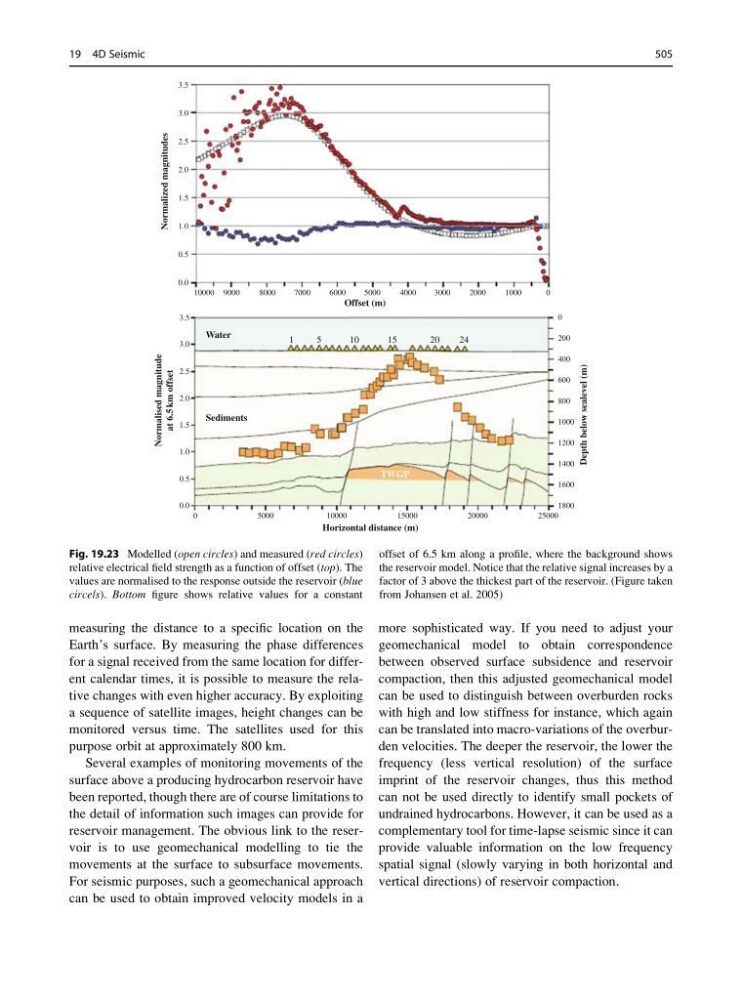
Fig. 19.23 Modelled (open circles) and measured (red circles)
relative electrical field strength as a function of offset (top). The
values are normalised to the response outside the reservoir (blue
circels). Bottom figure shows relative values for a constant
offset of 6.5 km along a profile, where the background shows
the reservoir model. Notice that the relative signal increases by a
factor of 3 above the thickest part of the reservoir. (Figure taken
from Johansen et al. 2005)
19 4D Seismic
505
Earth’s surface. By measuring the phase differences
for a signal received from the same location for different calendar times, it is possible to measure the relative changes with even higher accuracy. By exploiting
a sequence of satellite images, height changes can be
monitored versus time. The satellites used for this
purpose orbit at approximately 800 km.
Several examples of monitoring movements of the
surface above a producing hydrocarbon reservoir have
been reported, though there are of course limitations to
the detail of information such images can provide for
reservoir management. The obvious link to the reservoir is to use geomechanical modelling to tie the
movements at the surface to subsurface movements.
For seismic purposes, such a geomechanical approach
can be used to obtain improved velocity models in a
more sophisticated way. If you need to adjust your
geomechanical model to obtain correspondence
between observed surface subsidence and reservoir
compaction, then this adjusted geomechanical model
can be used to distinguish between overburden rocks
with high and low stiffness for instance, which again
can be translated into macro-variations of the overburden velocities. The deeper the reservoir, the lower the
frequency (less vertical resolution) of the surface
imprint of the reservoir changes, thus this method
can not be used directly to identify small pockets of
undrained hydrocarbons. However, it can be used as a
complementary tool for time-lapse seismic since it can
provide valuable information on the low frequency
spatial signal (slowly varying in both horizontal and
vertical directions) of reservoir compaction.
0
5000
10000
Horizontal distance (m)
Offset (m)
Water
1
5
10
15
TWGP
20
24
Sediments
Depth below sealevel (m)
Normalised magnitude
at 6.5
km offset
Normalized magnitudes
15000
20000
25000
1800
1600
0.0
0.5
1.0
1.5
2.0
2.5
3.0
3.5
0.0
10000 9000
8000
7000
6000
5000
4000
3000
2000
1000
0
0.5
1.0
1.5
2.0
2.5
3.0
3.5
1400
1200
1000
800
600
400
200
0
Fig. 19.23 Modelled (open circles) and measured (red circles)
relative electrical field strength as a function of offset (top). The
values are normalised to the response outside the reservoir (blue
circels). Bottom figure shows relative values for a constant
offset of 6.5 km along a profile, where the background shows
the reservoir model. Notice that the relative signal increases by a
factor of 3 above the thickest part of the reservoir. (Figure taken
from Johansen et al. 2005)
19 4D Seismic
505