

subdivision of the size range. It is then easy to see how
well sorted the sediments are, and whether the distribution of grain sizes is symmetrical, or perhaps bi- or
polymodal, i.e. with two, or more, maxima.
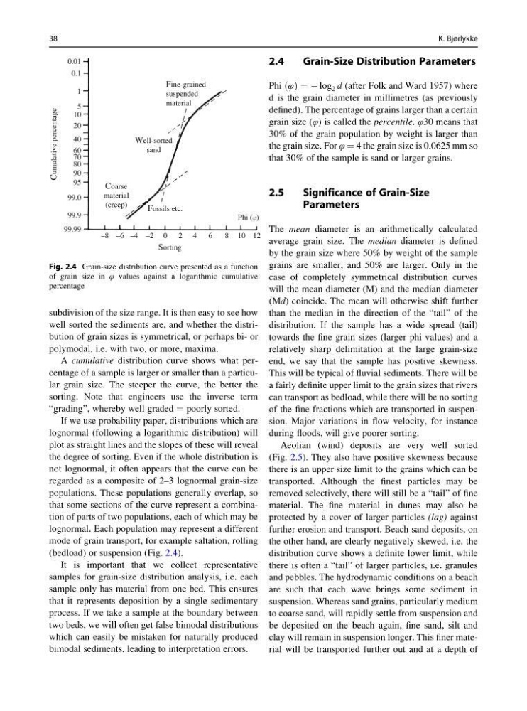
A cumulative distribution curve shows what percentage of a sample is larger or smaller than a particular grain size. The steeper the curve, the better the
sorting. Note that engineers use the inverse term
“grading”, whereby well graded ¼ poorly sorted.
If we use probability paper, distributions which are
lognormal (following a logarithmic distribution) will
plot as straight lines and the slopes of these will reveal
the degree of sorting. Even if the whole distribution is
not lognormal, it often appears that the curve can be
regarded as a composite of 2–3 lognormal grain-size
populations. These populations generally overlap, so
that some sections of the curve represent a combination of parts of two populations, each of which may be
lognormal. Each population may represent a different
mode of grain transport, for example saltation, rolling
(bedload) or suspension (Fig. 2.4).
It is important that we collect representative
samples for grain-size distribution analysis, i.e. each
sample only has material from one bed. This ensures
that it represents deposition by a single sedimentary
process. If we take a sample at the boundary between
two beds, we will often get false bimodal distributions
which can easily be mistaken for naturally produced
bimodal sediments, leading to interpretation errors.
2.4
Grain-Size Distribution Parameters
Phi φ
ð Þ ¼ À log 2 d (after Folk and Ward 1957) where
d is the grain diameter in millimetres (as previously
defined). The percentage of grains larger than a certain
grain size (φ) is called the percentile. φ30 means that
30% of the grain population by weight is larger than
the grain size. For φ ¼ 4 the grain size is 0.0625 mm so
that 30% of the sample is sand or larger grains.
2.5
Significance of Grain-Size
Parameters
The mean diameter is an arithmetically calculated
average grain size. The median diameter is defined
by the grain size where 50% by weight of the sample
grains are smaller, and 50% are larger. Only in the
case of completely symmetrical distribution curves
will the mean diameter (M) and the median diameter
(Md) coincide. The mean will otherwise shift further
than the median in the direction of the “tail” of the
distribution. If the sample has a wide spread (tail)
towards the fine grain sizes (larger phi values) and a
relatively sharp delimitation at the large grain-size
end, we say that the sample has positive skewness.
This will be typical of fluvial sediments. There will be
a fairly definite upper limit to the grain sizes that rivers
can transport as bedload, while there will be no sorting
of the fine fractions which are transported in suspension. Major variations in flow velocity, for instance
during floods, will give poorer sorting.
Aeolian (wind) deposits are very well sorted
(Fig. 2.5). They also have positive skewness because
there is an upper size limit to the grains which can be
transported. Although the finest particles may be
removed selectively, there will still be a “tail” of fine
material. The fine material in dunes may also be
protected by a cover of larger particles (lag) against
further erosion and transport. Beach sand deposits, on
the other hand, are clearly negatively skewed, i.e. the
distribution curve shows a definite lower limit, while
there is often a “tail” of larger particles, i.e. granules
and pebbles. The hydrodynamic conditions on a beach
are such that each wave brings some sediment in
suspension. Whereas sand grains, particularly medium
to coarse sand, will rapidly settle from suspension and
be deposited on the beach again, fine sand, silt and
clay will remain in suspension longer. This finer material will be transported further out and at a depth of
0.01
0.1
1
5
10
20
40
60
70
80
90
95
99.0
99.9
99.99
–8 –6 –4 –2 0 2 4
Sorting
Fossils etc.
Coarse
material
(creep)
Cumulative percentage
Well-sorted
sand
Fine-grained
suspended
material
6
Phi ( )
8 10 12
Fig. 2.4 Grain-size distribution curve presented as a function
of grain size in φ values against a logarithmic cumulative
percentage
38
K. Bjørlykke
well sorted the sediments are, and whether the distribution of grain sizes is symmetrical, or perhaps bi- or
polymodal, i.e. with two, or more, maxima.
A cumulative distribution curve shows what percentage of a sample is larger or smaller than a particular grain size. The steeper the curve, the better the
sorting. Note that engineers use the inverse term
“grading”, whereby well graded ¼ poorly sorted.
If we use probability paper, distributions which are
lognormal (following a logarithmic distribution) will
plot as straight lines and the slopes of these will reveal
the degree of sorting. Even if the whole distribution is
not lognormal, it often appears that the curve can be
regarded as a composite of 2–3 lognormal grain-size
populations. These populations generally overlap, so
that some sections of the curve represent a combination of parts of two populations, each of which may be
lognormal. Each population may represent a different
mode of grain transport, for example saltation, rolling
(bedload) or suspension (Fig. 2.4).
It is important that we collect representative
samples for grain-size distribution analysis, i.e. each
sample only has material from one bed. This ensures
that it represents deposition by a single sedimentary
process. If we take a sample at the boundary between
two beds, we will often get false bimodal distributions
which can easily be mistaken for naturally produced
bimodal sediments, leading to interpretation errors.
2.4
Grain-Size Distribution Parameters
Phi φ
ð Þ ¼ À log 2 d (after Folk and Ward 1957) where
d is the grain diameter in millimetres (as previously
defined). The percentage of grains larger than a certain
grain size (φ) is called the percentile. φ30 means that
30% of the grain population by weight is larger than
the grain size. For φ ¼ 4 the grain size is 0.0625 mm so
that 30% of the sample is sand or larger grains.
2.5
Significance of Grain-Size
Parameters
The mean diameter is an arithmetically calculated
average grain size. The median diameter is defined
by the grain size where 50% by weight of the sample
grains are smaller, and 50% are larger. Only in the
case of completely symmetrical distribution curves
will the mean diameter (M) and the median diameter
(Md) coincide. The mean will otherwise shift further
than the median in the direction of the “tail” of the
distribution. If the sample has a wide spread (tail)
towards the fine grain sizes (larger phi values) and a
relatively sharp delimitation at the large grain-size
end, we say that the sample has positive skewness.
This will be typical of fluvial sediments. There will be
a fairly definite upper limit to the grain sizes that rivers
can transport as bedload, while there will be no sorting
of the fine fractions which are transported in suspension. Major variations in flow velocity, for instance
during floods, will give poorer sorting.
Aeolian (wind) deposits are very well sorted
(Fig. 2.5). They also have positive skewness because
there is an upper size limit to the grains which can be
transported. Although the finest particles may be
removed selectively, there will still be a “tail” of fine
material. The fine material in dunes may also be
protected by a cover of larger particles (lag) against
further erosion and transport. Beach sand deposits, on
the other hand, are clearly negatively skewed, i.e. the
distribution curve shows a definite lower limit, while
there is often a “tail” of larger particles, i.e. granules
and pebbles. The hydrodynamic conditions on a beach
are such that each wave brings some sediment in
suspension. Whereas sand grains, particularly medium
to coarse sand, will rapidly settle from suspension and
be deposited on the beach again, fine sand, silt and
clay will remain in suspension longer. This finer material will be transported further out and at a depth of
0.01
0.1
1
5
10
20
40
60
70
80
90
95
99.0
99.9
99.99
–8 –6 –4 –2 0 2 4
Sorting
Fossils etc.
Coarse
material
(creep)
Cumulative percentage
Well-sorted
sand
Fine-grained
suspended
material
6
Phi ( )
8 10 12
Fig. 2.4 Grain-size distribution curve presented as a function
of grain size in φ values against a logarithmic cumulative
percentage
38
K. Bjørlykke