

representative for angles slightly higher than 0
) we
obtain the following approximate relationship
between the gradient and the Far-Near:
Far À Near ¼ R 30
ð Þ À R 0
ð Þ
¼ G Á sin
2 30
ð Þ ¼ G Á 0:25 ð18:29Þ
Solving for the background trend, that is when
ΔF ¼ 0, we obtain:
Near ¼
À20κ
8 À 5κ
Far À Near
ð
Þ
ð 18:30Þ
and hence:
η ¼
À20κ
8 À 5κ
ð18:31Þ
The slope of the background trend in the Near versus
Far-Near stack is 1/η, and this shows that we can in fact
estimate the expected background trend for uncalibrated
(but offset balanced) range limited stacks using the
modelled shale trends as illustrated above (Fig. 18.16).
This can be a useful task to verify the correct amplitude
balancing between near- and far-stack data during AVO
crossplot analysis.
Based on the shale model trends, we estimate the
value of η to be of the order 2.5. This means the
background trend of the shale in the AVO crossplot
is relatively flat, equaling À0.4, i.e., Far-Near ¼
À0.4Near. We observe indeed that the shale background trend is relatively flat (blue cloud in
Fig. 18.23). Using this background trend, the resulting
fluid factor attribute in Fig. 18.26 shows that both the
gas and the oil discoveries stand out as strong fluid
factor anomalies, whereas the background data is relatively weak.
We also estimate the difference between intercept
and gradient, which has been shown to be close to
ΔVs/Vs (Fatti et al. 1994, Avseth et al. 2005). This
attribute should not be significantly affected by pore
fluids, but very sensitive to lithology and cementation.
Figure 18.26 shows the fluid factor crossplot and line
superimposed with the ΔVs/Vs attribute for the seismic
line intersecting both well 1 and well 2. As expected,
both the gas and the oil discoveries show strong fluid
factors, whereas only well 1 (gas discovery) shows a
strong change in ΔVs/Vs at the top of the reservoir.
This tallies with the observations from the well log
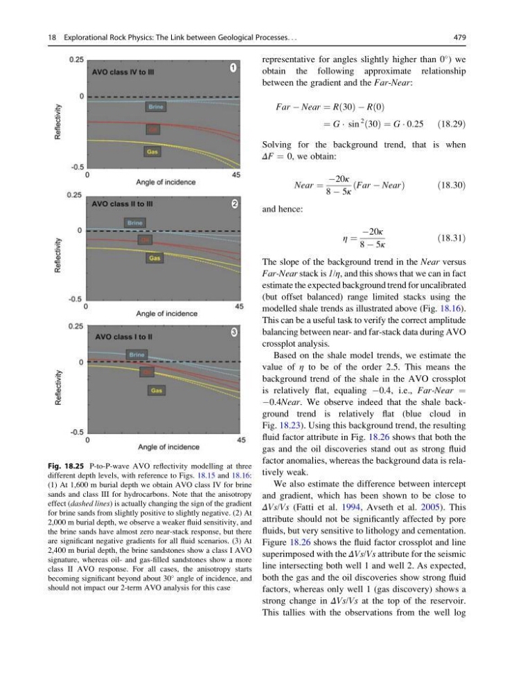
Fig. 18.25 P-to-P-wave AVO reflectivity modelling at three
different depth levels, with reference to Figs. 18.15 and 18.16:
(1) At 1,600 m burial depth we obtain AVO class IV for brine
sands and class III for hydrocarbons. Note that the anisotropy
effect (dashed lines) is actually changing the sign of the gradient
for brine sands from slightly positive to slightly negative. (2) At
2,000 m burial depth, we observe a weaker fluid sensitivity, and
the brine sands have almost zero near-stack response, but there
are significant negative gradients for all fluid scenarios. (3) At
2,400 m burial depth, the brine sandstones show a class I AVO
signature, whereas oil- and gas-filled sandstones show a more
class II AVO response. For all cases, the anisotropy starts
becoming significant beyond about 30
angle of incidence, and
should not impact our 2-term AVO analysis for this case
18 Explorational Rock Physics: The Link between Geological Processes. . .
479
) we
obtain the following approximate relationship
between the gradient and the Far-Near:
Far À Near ¼ R 30
ð Þ À R 0
ð Þ
¼ G Á sin
2 30
ð Þ ¼ G Á 0:25 ð18:29Þ
Solving for the background trend, that is when
ΔF ¼ 0, we obtain:
Near ¼
À20κ
8 À 5κ
Far À Near
ð
Þ
ð 18:30Þ
and hence:
η ¼
À20κ
8 À 5κ
ð18:31Þ
The slope of the background trend in the Near versus
Far-Near stack is 1/η, and this shows that we can in fact
estimate the expected background trend for uncalibrated
(but offset balanced) range limited stacks using the
modelled shale trends as illustrated above (Fig. 18.16).
This can be a useful task to verify the correct amplitude
balancing between near- and far-stack data during AVO
crossplot analysis.
Based on the shale model trends, we estimate the
value of η to be of the order 2.5. This means the
background trend of the shale in the AVO crossplot
is relatively flat, equaling À0.4, i.e., Far-Near ¼
À0.4Near. We observe indeed that the shale background trend is relatively flat (blue cloud in
Fig. 18.23). Using this background trend, the resulting
fluid factor attribute in Fig. 18.26 shows that both the
gas and the oil discoveries stand out as strong fluid
factor anomalies, whereas the background data is relatively weak.
We also estimate the difference between intercept
and gradient, which has been shown to be close to
ΔVs/Vs (Fatti et al. 1994, Avseth et al. 2005). This
attribute should not be significantly affected by pore
fluids, but very sensitive to lithology and cementation.
Figure 18.26 shows the fluid factor crossplot and line
superimposed with the ΔVs/Vs attribute for the seismic
line intersecting both well 1 and well 2. As expected,
both the gas and the oil discoveries show strong fluid
factors, whereas only well 1 (gas discovery) shows a
strong change in ΔVs/Vs at the top of the reservoir.
This tallies with the observations from the well log
Fig. 18.25 P-to-P-wave AVO reflectivity modelling at three
different depth levels, with reference to Figs. 18.15 and 18.16:
(1) At 1,600 m burial depth we obtain AVO class IV for brine
sands and class III for hydrocarbons. Note that the anisotropy
effect (dashed lines) is actually changing the sign of the gradient
for brine sands from slightly positive to slightly negative. (2) At
2,000 m burial depth, we observe a weaker fluid sensitivity, and
the brine sands have almost zero near-stack response, but there
are significant negative gradients for all fluid scenarios. (3) At
2,400 m burial depth, the brine sandstones show a class I AVO
signature, whereas oil- and gas-filled sandstones show a more
class II AVO response. For all cases, the anisotropy starts
becoming significant beyond about 30
angle of incidence, and
should not impact our 2-term AVO analysis for this case
18 Explorational Rock Physics: The Link between Geological Processes. . .
479