

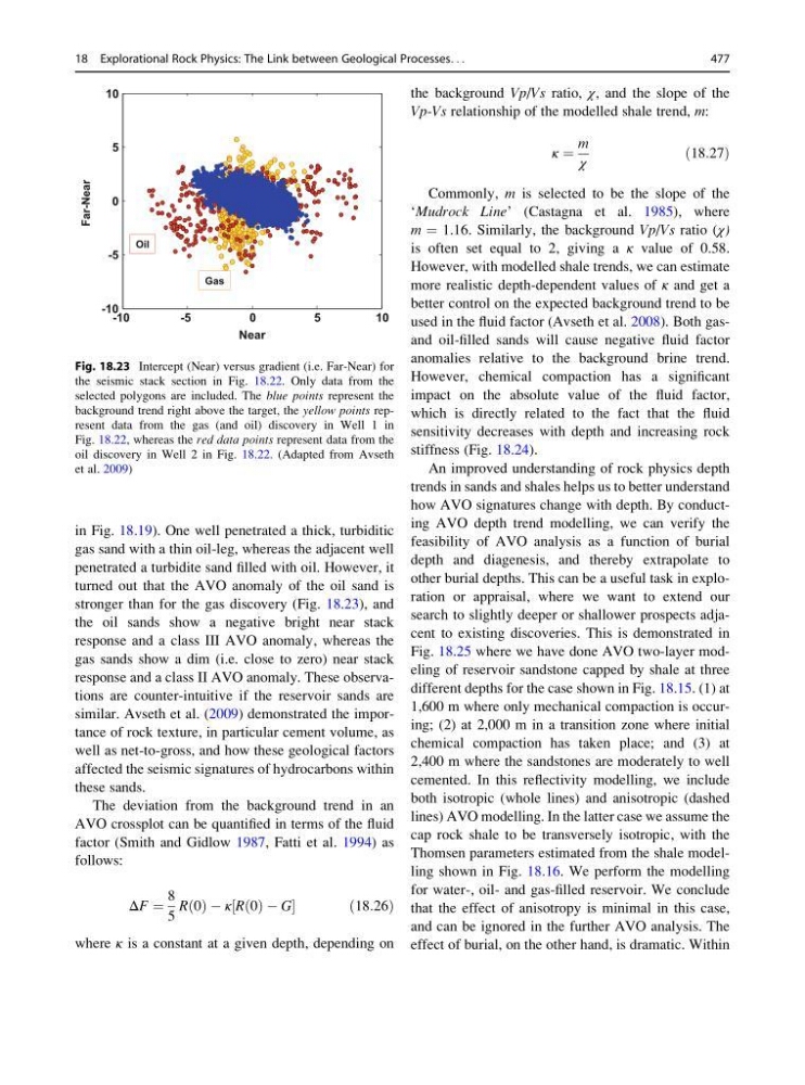
in Fig. 18.19). One well penetrated a thick, turbiditic
gas sand with a thin oil-leg, whereas the adjacent well
penetrated a turbidite sand filled with oil. However, it
turned out that the AVO anomaly of the oil sand is
stronger than for the gas discovery (Fig. 18.23), and
the oil sands show a negative bright near stack
response and a class III AVO anomaly, whereas the
gas sands show a dim (i.e. close to zero) near stack
response and a class II AVO anomaly. These observations are counter-intuitive if the reservoir sands are
similar. Avseth et al. (2009) demonstrated the importance of rock texture, in particular cement volume, as
well as net-to-gross, and how these geological factors
affected the seismic signatures of hydrocarbons within
these sands.
The deviation from the background trend in an
AVO crossplot can be quantified in terms of the fluid
factor (Smith and Gidlow 1987, Fatti et al. 1994) as
follows:
ΔF ¼
8
5
R 0
ð Þ À κ R 0
ð Þ À G
½
ð 18:26Þ
where κ is a constant at a given depth, depending on
the background Vp/Vs ratio, χ, and the slope of the
Vp-Vs relationship of the modelled shale trend, m:
κ ¼
m
χ
ð18:27Þ
Commonly, m is selected to be the slope of the
‘Mudrock Line’ (Castagna et al. 1985), where
m ¼ 1.16. Similarly, the background Vp/Vs ratio (χ)
is often set equal to 2, giving a κ value of 0.58.
However, with modelled shale trends, we can estimate
more realistic depth-dependent values of κ and get a
better control on the expected background trend to be
used in the fluid factor (Avseth et al. 2008). Both gasand oil-filled sands will cause negative fluid factor
anomalies relative to the background brine trend.
However, chemical compaction has a significant
impact on the absolute value of the fluid factor,
which is directly related to the fact that the fluid
sensitivity decreases with depth and increasing rock
stiffness (Fig. 18.24).
An improved understanding of rock physics depth
trends in sands and shales helps us to better understand
how AVO signatures change with depth. By conducting AVO depth trend modelling, we can verify the
feasibility of AVO analysis as a function of burial
depth and diagenesis, and thereby extrapolate to
other burial depths. This can be a useful task in exploration or appraisal, where we want to extend our
search to slightly deeper or shallower prospects adjacent to existing discoveries. This is demonstrated in
Fig. 18.25 where we have done AVO two-layer modeling of reservoir sandstone capped by shale at three
different depths for the case shown in Fig. 18.15. (1) at
1,600 m where only mechanical compaction is occuring; (2) at 2,000 m in a transition zone where initial
chemical compaction has taken place; and (3) at
2,400 m where the sandstones are moderately to well
cemented. In this reflectivity modelling, we include
both isotropic (whole lines) and anisotropic (dashed
lines) AVO modelling. In the latter case we assume the
cap rock shale to be transversely isotropic, with the
Thomsen parameters estimated from the shale modelling shown in Fig. 18.16. We perform the modelling
for water-, oil- and gas-filled reservoir. We conclude
that the effect of anisotropy is minimal in this case,
and can be ignored in the further AVO analysis. The
effect of burial, on the other hand, is dramatic. Within
-10
-5
0
5
10
-10
-5
0
5
10
Near
Far-Near
Oil
Gas
Fig. 18.23 Intercept (Near) versus gradient (i.e. Far-Near) for
the seismic stack section in Fig. 18.22. Only data from the
selected polygons are included. The blue points represent the
background trend right above the target, the yellow points represent data from the gas (and oil) discovery in Well 1 in
Fig. 18.22, whereas the red data points represent data from the
oil discovery in Well 2 in Fig. 18.22. (Adapted from Avseth
et al. 2009)
18 Explorational Rock Physics: The Link between Geological Processes. . .
477
gas sand with a thin oil-leg, whereas the adjacent well
penetrated a turbidite sand filled with oil. However, it
turned out that the AVO anomaly of the oil sand is
stronger than for the gas discovery (Fig. 18.23), and
the oil sands show a negative bright near stack
response and a class III AVO anomaly, whereas the
gas sands show a dim (i.e. close to zero) near stack
response and a class II AVO anomaly. These observations are counter-intuitive if the reservoir sands are
similar. Avseth et al. (2009) demonstrated the importance of rock texture, in particular cement volume, as
well as net-to-gross, and how these geological factors
affected the seismic signatures of hydrocarbons within
these sands.
The deviation from the background trend in an
AVO crossplot can be quantified in terms of the fluid
factor (Smith and Gidlow 1987, Fatti et al. 1994) as
follows:
ΔF ¼
8
5
R 0
ð Þ À κ R 0
ð Þ À G
½
ð 18:26Þ
where κ is a constant at a given depth, depending on
the background Vp/Vs ratio, χ, and the slope of the
Vp-Vs relationship of the modelled shale trend, m:
κ ¼
m
χ
ð18:27Þ
Commonly, m is selected to be the slope of the
‘Mudrock Line’ (Castagna et al. 1985), where
m ¼ 1.16. Similarly, the background Vp/Vs ratio (χ)
is often set equal to 2, giving a κ value of 0.58.
However, with modelled shale trends, we can estimate
more realistic depth-dependent values of κ and get a
better control on the expected background trend to be
used in the fluid factor (Avseth et al. 2008). Both gasand oil-filled sands will cause negative fluid factor
anomalies relative to the background brine trend.
However, chemical compaction has a significant
impact on the absolute value of the fluid factor,
which is directly related to the fact that the fluid
sensitivity decreases with depth and increasing rock
stiffness (Fig. 18.24).
An improved understanding of rock physics depth
trends in sands and shales helps us to better understand
how AVO signatures change with depth. By conducting AVO depth trend modelling, we can verify the
feasibility of AVO analysis as a function of burial
depth and diagenesis, and thereby extrapolate to
other burial depths. This can be a useful task in exploration or appraisal, where we want to extend our
search to slightly deeper or shallower prospects adjacent to existing discoveries. This is demonstrated in
Fig. 18.25 where we have done AVO two-layer modeling of reservoir sandstone capped by shale at three
different depths for the case shown in Fig. 18.15. (1) at
1,600 m where only mechanical compaction is occuring; (2) at 2,000 m in a transition zone where initial
chemical compaction has taken place; and (3) at
2,400 m where the sandstones are moderately to well
cemented. In this reflectivity modelling, we include
both isotropic (whole lines) and anisotropic (dashed
lines) AVO modelling. In the latter case we assume the
cap rock shale to be transversely isotropic, with the
Thomsen parameters estimated from the shale modelling shown in Fig. 18.16. We perform the modelling
for water-, oil- and gas-filled reservoir. We conclude
that the effect of anisotropy is minimal in this case,
and can be ignored in the further AVO analysis. The
effect of burial, on the other hand, is dramatic. Within
-10
-5
0
5
10
-10
-5
0
5
10
Near
Far-Near
Oil
Gas
Fig. 18.23 Intercept (Near) versus gradient (i.e. Far-Near) for
the seismic stack section in Fig. 18.22. Only data from the
selected polygons are included. The blue points represent the
background trend right above the target, the yellow points represent data from the gas (and oil) discovery in Well 1 in
Fig. 18.22, whereas the red data points represent data from the
oil discovery in Well 2 in Fig. 18.22. (Adapted from Avseth
et al. 2009)
18 Explorational Rock Physics: The Link between Geological Processes. . .
477