

48
Statistical Methods for Estimating Petroleum Resources
higher (unless there is only one pool). In the case of more than one pool,
the probability can be obtained from the distribution of the largest
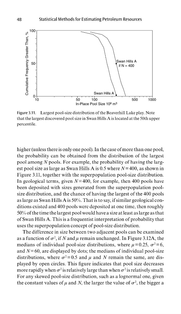
pool among N pools. For example, the probability of having the largest pool size as large as Swan Hills A is 0.5 where N = 400, as shown in
Figure 3.11, together with the superpopulation pool-size distribution.
In geological terms, given N = 400, for example, then 400 pools have
been deposited with sizes generated from the superpopulation poolsize distribution, and the chance of having the largest of the 400 pools
as large as Swan Hills A is 50%. That is to say, if similar geological conditions existed and 400 pools were deposited at one time, then roughly
50% of the time the largest pool would have a size at least as large as that
of Swan Hills A. This is a frequentist interpretation of probability that
uses the superpopulation concept of pool-size distribution.
The difference in size between two adjacent pools can be examined
as a function of σ
2 , if N and μ remain unchanged. In Figure 3.12A, the
medians of individual pool-size distributions, where μ = 0.25, σ
2 = 6,
and N = 60, are displayed by dots; the medians of individual pool-size
distributions, where σ
2 = 0.5 and μ and N remain the same, are displayed by open circles. This fi gure indicates that pool size decreases
more rapidly when σ
2 is relatively large than when σ
2 is relatively small.
For any skewed pool-size distribution, such as a lognormal one, given
the constant values of μ and N, the larger the value of σ
2 , the bigger a
Swan Hills A
Swan Hills A
if N = 400
0
50
100
Cumulative Frequency Greater Than, %
10
50
100
500
1000
In-Place Pool Size 10 6 m 3
Figure 3.11. Largest pool-size distribution of the Beaverhill Lake play. Note
that the largest discovered pool size in Swan Hills A is located at the 50th upper
percentile.
Statistical Methods for Estimating Petroleum Resources
higher (unless there is only one pool). In the case of more than one pool,
the probability can be obtained from the distribution of the largest
pool among N pools. For example, the probability of having the largest pool size as large as Swan Hills A is 0.5 where N = 400, as shown in
Figure 3.11, together with the superpopulation pool-size distribution.
In geological terms, given N = 400, for example, then 400 pools have
been deposited with sizes generated from the superpopulation poolsize distribution, and the chance of having the largest of the 400 pools
as large as Swan Hills A is 50%. That is to say, if similar geological conditions existed and 400 pools were deposited at one time, then roughly
50% of the time the largest pool would have a size at least as large as that
of Swan Hills A. This is a frequentist interpretation of probability that
uses the superpopulation concept of pool-size distribution.
The difference in size between two adjacent pools can be examined
as a function of σ
2 , if N and μ remain unchanged. In Figure 3.12A, the
medians of individual pool-size distributions, where μ = 0.25, σ
2 = 6,
and N = 60, are displayed by dots; the medians of individual pool-size
distributions, where σ
2 = 0.5 and μ and N remain the same, are displayed by open circles. This fi gure indicates that pool size decreases
more rapidly when σ
2 is relatively large than when σ
2 is relatively small.
For any skewed pool-size distribution, such as a lognormal one, given
the constant values of μ and N, the larger the value of σ
2 , the bigger a
Swan Hills A
Swan Hills A
if N = 400
0
50
100
Cumulative Frequency Greater Than, %
10
50
100
500
1000
In-Place Pool Size 10 6 m 3
Figure 3.11. Largest pool-size distribution of the Beaverhill Lake play. Note
that the largest discovered pool size in Swan Hills A is located at the 50th upper
percentile.