

198
Appendix A
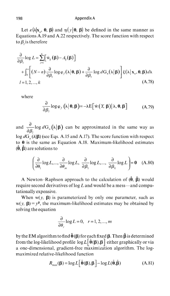
Let « (l|x n , , ) and h ( y | , ) be defi ned in the same manner as
Equations A.19 and A.22 respectively. The score function with respect
to b l is therefore
w l
l
j l
l
=
∞
∂
=
−
∂
∂
∂
+
−
+
∂
∂
=
∑
∫
1
0
log
w
log
,
log G
, ,
1, 2, ...,
( )
( )
(
)
(
)
(
)
( )
n
lj
lj
j
l
f
n
n
l
l
L
A
N n
d
d
l
k
x
b
b
b


(A.78)
where
(
)
( )
log
,
E w ,
, ,
f
l
Y
w l
l
l
∂
= −
∂b


(A.79)
and
( )
log G n
l
d
l
∂
∂b
 can be approximated in the same way as
log dG n (l|) (see Eqs. A.15 and A.17). The score function with respect
to is the same as Equation A.18. Maximum-likelihood estimates
( ˆ ,  ˆ ) are solutions to
1
1
log ,...,
log ,
log ,...,
log
m
k
L
L
L
L
u
∂
∂
∂
∂
=
∂
∂
∂
∂
0
u
b
b
(A.80)
A Newton–Raphson approach to the calculation of ( ˆ ,  ˆ ) would
require second derivatives of log L and would be a mess—and computationally expensive.
When w( y, ) is parameterized by only one parameter, such as
w( y, ) 5 y

, the maximum-likelihood estimates may be obtained by
solving the equation
log
0,
1, 2, ...,
r
L
r
m
∂
=
=
∂u
by the EM algorithm to fi nd ˆ () for each fi xed . Then  ˆ is determined
from the log-likelihood profi le
ˆ
log
( ),
L   either graphically or via
a one-dimensional, gradient-free maximization algorithm. The logmaximized relative-likelihood function
=
−
max
ˆ
ˆˆ
( ) log
( ),
log ( , )
R
L
L


(A.81)
Appendix A
Let « (l|x n , , ) and h ( y | , ) be defi ned in the same manner as
Equations A.19 and A.22 respectively. The score function with respect
to b l is therefore
w l
l
j l
l
=
∞
∂
=
−
∂
∂
∂
+
−
+
∂
∂
=
∑
∫
1
0
log
w
log
,
log G
, ,
1, 2, ...,
( )
( )
(
)
(
)
(
)
( )
n
lj
lj
j
l
f
n
n
l
l
L
A
N n
d
d
l
k
x
b
b
b


(A.78)
where
(
)
( )
log
,
E w ,
, ,
f
l
Y
w l
l
l
∂
= −
∂b


(A.79)
and
( )
log G n
l
d
l
∂
∂b
 can be approximated in the same way as
log dG n (l|) (see Eqs. A.15 and A.17). The score function with respect
to is the same as Equation A.18. Maximum-likelihood estimates
( ˆ ,  ˆ ) are solutions to
1
1
log ,...,
log ,
log ,...,
log
m
k
L
L
L
L
u
∂
∂
∂
∂
=
∂
∂
∂
∂
0
u
b
b
(A.80)
A Newton–Raphson approach to the calculation of ( ˆ ,  ˆ ) would
require second derivatives of log L and would be a mess—and computationally expensive.
When w( y, ) is parameterized by only one parameter, such as
w( y, ) 5 y

, the maximum-likelihood estimates may be obtained by
solving the equation
log
0,
1, 2, ...,
r
L
r
m
∂
=
=
∂u
by the EM algorithm to fi nd ˆ () for each fi xed . Then  ˆ is determined
from the log-likelihood profi le
ˆ
log
( ),
L   either graphically or via
a one-dimensional, gradient-free maximization algorithm. The logmaximized relative-likelihood function
=
−
max
ˆ
ˆˆ
( ) log
( ),
log ( , )
R
L
L


(A.81)