

168
Statistical Methods for Estimating Petroleum Resources
Furthermore, Coustau (1981) adopted Zipf’s law (Zipf, 1949) and
stated that
S m / S n = (n / m)
k
(7.19)
where S m is the pool size of rank m, S n is the pool size of rank n, and k is
a constant.
Taking k = 1 as an example, Equation 7.19 states that the largest pool
size is twice as large as the rank 2 pool, and three times the size of the
rank 3 pool, and so on. This implies that if the ratios between two adjacent ranked pools do not approximate the constant, then additional
undiscovered pools might exist in size rank between the two. Coustau
(1981) displayed pool-size-by-rank on a doubly logarithmic diagram.
In this approach, the pools were arranged according to their descending order of size, and a rank was allocated to each of the pools. This
suggested that if the lines declined with a gentle slope, then the play had
a “dispersed habitat”; whereas if the lines declined with a steep slope,
then the play had a “concentrated habitat.” Dispersed habitat and
concentrated habitat are terms defi ned by Klemme (1986). Comparisons
between the methods of Zipf’s law, geochemical mass balance, and the
PETRIMES discovery process method were published by Coustau
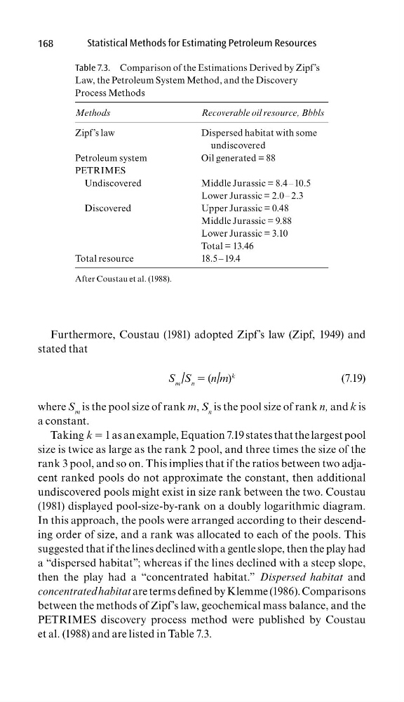
et al. (1988) and are listed in Table 7.3.
Table 7.3. Comparison of the Estimations Derived by Zipf’s
Law, the Petroleum System Method, and the Discovery
Process Methods
Methods
Recoverable oil resource, Bbbls
Zipf’s law
Dispersed habitat with some
undiscovered
Petroleum system
Oil generated = 88
PETRIMES
Undiscovered
Middle Jurassic = 8.4 – 10.5
Lower Jurassic = 2.0 – 2.3
Discovered
Upper Jurassic = 0.48
Middle Jurassic = 9.88
Lower Jurassic = 3.10
Total = 13.46
Total resource
18.5 – 19.4
After Coustau et al. (1988).
Statistical Methods for Estimating Petroleum Resources
Furthermore, Coustau (1981) adopted Zipf’s law (Zipf, 1949) and
stated that
S m / S n = (n / m)
k
(7.19)
where S m is the pool size of rank m, S n is the pool size of rank n, and k is
a constant.
Taking k = 1 as an example, Equation 7.19 states that the largest pool
size is twice as large as the rank 2 pool, and three times the size of the
rank 3 pool, and so on. This implies that if the ratios between two adjacent ranked pools do not approximate the constant, then additional
undiscovered pools might exist in size rank between the two. Coustau
(1981) displayed pool-size-by-rank on a doubly logarithmic diagram.
In this approach, the pools were arranged according to their descending order of size, and a rank was allocated to each of the pools. This
suggested that if the lines declined with a gentle slope, then the play had
a “dispersed habitat”; whereas if the lines declined with a steep slope,
then the play had a “concentrated habitat.” Dispersed habitat and
concentrated habitat are terms defi ned by Klemme (1986). Comparisons
between the methods of Zipf’s law, geochemical mass balance, and the
PETRIMES discovery process method were published by Coustau
et al. (1988) and are listed in Table 7.3.
Table 7.3. Comparison of the Estimations Derived by Zipf’s
Law, the Petroleum System Method, and the Discovery
Process Methods
Methods
Recoverable oil resource, Bbbls
Zipf’s law
Dispersed habitat with some
undiscovered
Petroleum system
Oil generated = 88
PETRIMES
Undiscovered
Middle Jurassic = 8.4 – 10.5
Lower Jurassic = 2.0 – 2.3
Discovered
Upper Jurassic = 0.48
Middle Jurassic = 9.88
Lower Jurassic = 3.10
Total = 13.46
Total resource
18.5 – 19.4
After Coustau et al. (1988).