

Other Assessment Methods—An Overview
163
where F i (w) is the number of fi elds found in the i th class by w exploratory wells, F (∞) is the total number of fi elds, W is the number of wells,
C i is the drilling effi ciency for the i th size class, B is the basin area to be
tested, and A i is the average areal extent of fi elds in the i th size class.
The advantages of the method are twofold: (1) it is suitable for the
evaluation of basins and (2) it provides quick estimates of the number and sizes of fi elds in a basin, and results can be used in economic
research. The disadvantages are also twofold: (1) when estimating
unknown population parameters, standard statistical methods do not
apply for measuring uncertainty; and (2) the basin area to be tested, B,
is diffi cult to estimate and is directly infl uenced by the number of fi elds
to be estimated.
Take the Permian Basin of West Texas and southeastern New
Mexico (Drew et al., 1980) as an example. The size class 10 has the following parameters: average areal extent of fi elds, 2.2 sq. mi.; cumulative exploratory wells through 1960, 14,243; and number of discoveries
in size class 10 in the 0 to 5000-ft. interval through 1960, 59. The basin
area is equal to 100,000 sq. mi., so the ultimate number of fi elds is 127. If
the basin area were reduced by 50% (i.e., to 50,000 sq. mi.), the ultimate
number of fi elds would be reduced to 83.
Bickel, Nair, and Wang’s Method
Bickel’s method (Bickel et al., 1992) is described as follows. Let
U = {x 1 , . . . , x N } denote a fi nite population of N members and let Y j be
a characteristic associated with x j , j = 1, . . . , N. Let S n = (x i1 , . . . , x in )
be an ordered sample of size n that is selected successively without
replacement and with probability proportional to some measure of size
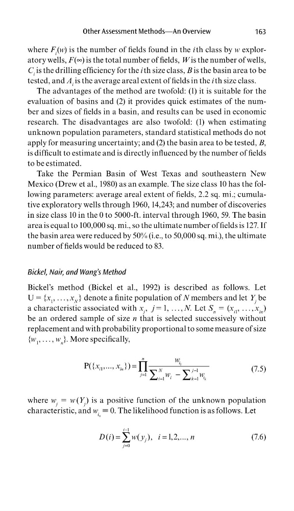
{w 1 , . . . , w n }. More specifi cally,
1
1
1
1
1
1
P({ ,..., })
k
n
i
i
i n
N
j
j
i
i
i
k
w
x
x
w
w
−
=
=
=
=
−
∏ ∑
∑
(7.5)
where w j = w (Y j ) is a positive function of the unknown population
characteristic, and w i 0 ≡ 0. The likelihood function is as follows. Let
1
0
( )
( ),
1,2,...,
i
j
j
D i
w y
i
n
−
=
=
=
∑
(7.6)
163
where F i (w) is the number of fi elds found in the i th class by w exploratory wells, F (∞) is the total number of fi elds, W is the number of wells,
C i is the drilling effi ciency for the i th size class, B is the basin area to be
tested, and A i is the average areal extent of fi elds in the i th size class.
The advantages of the method are twofold: (1) it is suitable for the
evaluation of basins and (2) it provides quick estimates of the number and sizes of fi elds in a basin, and results can be used in economic
research. The disadvantages are also twofold: (1) when estimating
unknown population parameters, standard statistical methods do not
apply for measuring uncertainty; and (2) the basin area to be tested, B,
is diffi cult to estimate and is directly infl uenced by the number of fi elds
to be estimated.
Take the Permian Basin of West Texas and southeastern New
Mexico (Drew et al., 1980) as an example. The size class 10 has the following parameters: average areal extent of fi elds, 2.2 sq. mi.; cumulative exploratory wells through 1960, 14,243; and number of discoveries
in size class 10 in the 0 to 5000-ft. interval through 1960, 59. The basin
area is equal to 100,000 sq. mi., so the ultimate number of fi elds is 127. If
the basin area were reduced by 50% (i.e., to 50,000 sq. mi.), the ultimate
number of fi elds would be reduced to 83.
Bickel, Nair, and Wang’s Method
Bickel’s method (Bickel et al., 1992) is described as follows. Let
U = {x 1 , . . . , x N } denote a fi nite population of N members and let Y j be
a characteristic associated with x j , j = 1, . . . , N. Let S n = (x i1 , . . . , x in )
be an ordered sample of size n that is selected successively without
replacement and with probability proportional to some measure of size
{w 1 , . . . , w n }. More specifi cally,
1
1
1
1
1
1
P({ ,..., })
k
n
i
i
i n
N
j
j
i
i
i
k
w
x
x
w
w
−
=
=
=
=
−
∏ ∑
∑
(7.5)
where w j = w (Y j ) is a positive function of the unknown population
characteristic, and w i 0 ≡ 0. The likelihood function is as follows. Let
1
0
( )
( ),
1,2,...,
i
j
j
D i
w y
i
n
−
=
=
=
∑
(7.6)