

Evaluating Conceptual Plays
135
probability of having at least r pools is provided. The results of the two
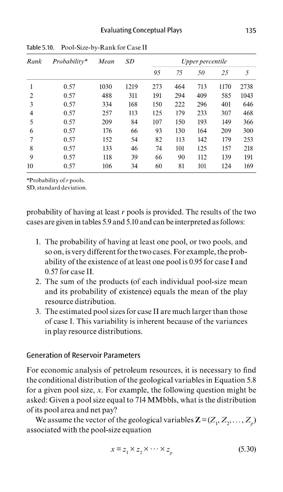
cases are given in tables 5.9 and 5.10 and can be interpreted as follows:
The probability of having at least one pool, or two pools, and
1.
so on, is very different for the two cases. For example, the probability of the existence of at least one pool is 0.95 for case I and
0.57 for case II.
The sum of the products (of each individual pool-size mean
2.
and its probability of existence) equals the mean of the play
resource distribution.
The estimated pool sizes for case II are much larger than those
3.
of case I. This variability is inherent because of the variances
in play resource distributions.
Generation of Reservoir Parameters
For economic analysis of petroleum resources, it is necessary to fi nd
the conditional distribution of the geological variables in Equation 5.8
for a given pool size, x. For example, the following question might be
asked: Given a pool size equal to 714 MMbbls, what is the distribution
of its pool area and net pay?
We assume the vector of the geological variables Z = (Z 1 , Z 2 , . . . , Z p )
associated with the pool-size equation
x = z 1 × z 2 × · · · × z p
(5.30)
Table 5.10. Pool-Size-by-Rank for Case II
Rank
Probability*
Mean
SD
Upper percentile
95
75
50
25
5
1
0 . 5 7
1 0 3 0
1 2 1 9
2 7 3
4 6 4
7 1 3
1 1 7 0 2 7 3 8
2
0 . 5 7
4 8 8
3 1 1
1 9 1
2 9 4
4 0 9
5 8 5 1 0 4 3
3
0.57
334
168
150
222
296
401
646
4
0 . 5 7
2 5 7
1 1 3
1 2 5
1 7 9
2 3 3
3 0 7
4 6 8
5
0 . 5 7
2 0 9
8 4
1 0 7
1 5 0
1 9 3
1 4 9
3 6 6
6
0 . 5 7
1 7 6
6 6
9 3
1 3 0
1 6 4
2 0 9
3 0 0
7
0 . 5 7
1 5 2
5 4
8 2
1 1 3
1 4 2
1 7 9
2 5 3
8
0 . 5 7
1 3 3
4 6
7 4
1 0 1
1 2 5
1 5 7
2 1 8
9
0.57
118
39
66
90
112
139
191
10
0.57
106
34
60
81
101
124
169
*Probability of r pools.
SD, standard deviation.
135
probability of having at least r pools is provided. The results of the two
cases are given in tables 5.9 and 5.10 and can be interpreted as follows:
The probability of having at least one pool, or two pools, and
1.
so on, is very different for the two cases. For example, the probability of the existence of at least one pool is 0.95 for case I and
0.57 for case II.
The sum of the products (of each individual pool-size mean
2.
and its probability of existence) equals the mean of the play
resource distribution.
The estimated pool sizes for case II are much larger than those
3.
of case I. This variability is inherent because of the variances
in play resource distributions.
Generation of Reservoir Parameters
For economic analysis of petroleum resources, it is necessary to fi nd
the conditional distribution of the geological variables in Equation 5.8
for a given pool size, x. For example, the following question might be
asked: Given a pool size equal to 714 MMbbls, what is the distribution
of its pool area and net pay?
We assume the vector of the geological variables Z = (Z 1 , Z 2 , . . . , Z p )
associated with the pool-size equation
x = z 1 × z 2 × · · · × z p
(5.30)
Table 5.10. Pool-Size-by-Rank for Case II
Rank
Probability*
Mean
SD
Upper percentile
95
75
50
25
5
1
0 . 5 7
1 0 3 0
1 2 1 9
2 7 3
4 6 4
7 1 3
1 1 7 0 2 7 3 8
2
0 . 5 7
4 8 8
3 1 1
1 9 1
2 9 4
4 0 9
5 8 5 1 0 4 3
3
0.57
334
168
150
222
296
401
646
4
0 . 5 7
2 5 7
1 1 3
1 2 5
1 7 9
2 3 3
3 0 7
4 6 8
5
0 . 5 7
2 0 9
8 4
1 0 7
1 5 0
1 9 3
1 4 9
3 6 6
6
0 . 5 7
1 7 6
6 6
9 3
1 3 0
1 6 4
2 0 9
3 0 0
7
0 . 5 7
1 5 2
5 4
8 2
1 1 3
1 4 2
1 7 9
2 5 3
8
0 . 5 7
1 3 3
4 6
7 4
1 0 1
1 2 5
1 5 7
2 1 8
9
0.57
118
39
66
90
112
139
191
10
0.57
106
34
60
81
101
124
169
*Probability of r pools.
SD, standard deviation.