

126
Statistical Methods for Estimating Petroleum Resources
If the geological variables are approximated by lognormal distributions with parameters μ and s
2 , and if they are independent, then
ln x = ln c + S ln Z i
(5.15)
is normally distributed with μ ˆ = 2.882 and s ˆ
2 = 2.5, and its density is
given by
2
1
l n
1
( )
exp 2
2
x
h x
x
−
=
−
m
s
s p
(5.16)
where x is the pool size in MMbbls.
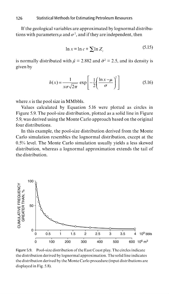
Values calculated by Equation 5.16 were plotted as circles in
Figure 5.9. The pool-size distribution, plotted as a solid line in Figure
5.9, was derived using the Monte Carlo approach based on the original
four distributions.
In this example, the pool-size distribution derived from the Monte
Carlo simulation resembles the lognormal distribution, except at the
0.5% level. The Monte Carlo simulation usually yields a less skewed
distribution, whereas a lognormal approximation extends the tail of
the distribution.
0
0
0
50
100
100
200
CUMULATIVE FREQUENCY
GREATER THAN, %
300
400
500
600
0.5
1
1.5
2
2.5
3
3.5
4 10
9 bbls
10
6 m
3
Figure 5.9. Pool-size distribution of the East Coast play. The circles indicate
the distribution derived by lognormal approximation. The solid line indicates
the distribution derived by the Monte Carlo procedure (input distributions are
displayed in Fig. 5.8).
Statistical Methods for Estimating Petroleum Resources
If the geological variables are approximated by lognormal distributions with parameters μ and s
2 , and if they are independent, then
ln x = ln c + S ln Z i
(5.15)
is normally distributed with μ ˆ = 2.882 and s ˆ
2 = 2.5, and its density is
given by
2
1
l n
1
( )
exp 2
2
x
h x
x
−
=
−
m
s
s p
(5.16)
where x is the pool size in MMbbls.
Values calculated by Equation 5.16 were plotted as circles in
Figure 5.9. The pool-size distribution, plotted as a solid line in Figure
5.9, was derived using the Monte Carlo approach based on the original
four distributions.
In this example, the pool-size distribution derived from the Monte
Carlo simulation resembles the lognormal distribution, except at the
0.5% level. The Monte Carlo simulation usually yields a less skewed
distribution, whereas a lognormal approximation extends the tail of
the distribution.
0
0
0
50
100
100
200
CUMULATIVE FREQUENCY
GREATER THAN, %
300
400
500
600
0.5
1
1.5
2
2.5
3
3.5
4 10
9 bbls
10
6 m
3
Figure 5.9. Pool-size distribution of the East Coast play. The circles indicate
the distribution derived by lognormal approximation. The solid line indicates
the distribution derived by the Monte Carlo procedure (input distributions are
displayed in Fig. 5.8).