

Prediction Model of Converter Oxygen Consumption Based on Recursive …
107
At this point, the recursion depth is 2, which has reached the division stop condition. The y O2 ’s distribution concentration corresponding to each feature space is also
difficult to be greatly improved. It indicates that the stopping condition is appropriate. With the increase of the division depth, the number of samples contained in
the feature space gradually decreases, and the corresponding y O2 s’ MSEs gradually
decrease and their distribution becomes more and more concentrated to facilitate the
fitting of the prediction model.
Feature Variable Selection and Analysis
Feature variable selection needs to be performed in each feature subspace, namely,
S 1,1 , S 1,2 , S 2,1 , S 2,2 . Since the feature selection method on each subspace is the same,
here is only the case of feature selection on subspace S 2,1 for illustration. Here,
MLP is selected as the prediction model, and 12 feature variable combinations and
the corresponding trained MLPs are obtained based on the RFE algorithm. The
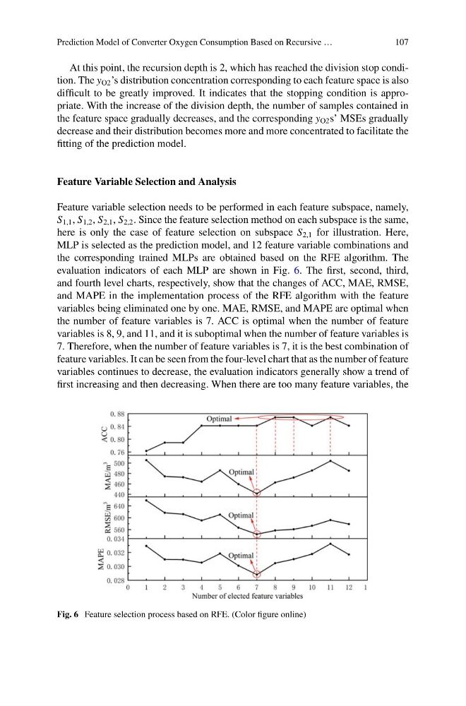
evaluation indicators of each MLP are shown in Fig. 6. The first, second, third,
and fourth level charts, respectively, show that the changes of ACC, MAE, RMSE,
and MAPE in the implementation process of the RFE algorithm with the feature
variables being eliminated one by one. MAE, RMSE, and MAPE are optimal when
the number of feature variables is 7. ACC is optimal when the number of feature
variables is 8, 9, and 11, and it is suboptimal when the number of feature variables is
7. Therefore, when the number of feature variables is 7, it is the best combination of
feature variables. It can be seen from the four-level chart that as the number of feature
variables continues to decrease, the evaluation indicators generally show a trend of
first increasing and then decreasing. When there are too many feature variables, the
Fig. 6 Feature selection process based on RFE. (Color figure online)
107
At this point, the recursion depth is 2, which has reached the division stop condition. The y O2 ’s distribution concentration corresponding to each feature space is also
difficult to be greatly improved. It indicates that the stopping condition is appropriate. With the increase of the division depth, the number of samples contained in
the feature space gradually decreases, and the corresponding y O2 s’ MSEs gradually
decrease and their distribution becomes more and more concentrated to facilitate the
fitting of the prediction model.
Feature Variable Selection and Analysis
Feature variable selection needs to be performed in each feature subspace, namely,
S 1,1 , S 1,2 , S 2,1 , S 2,2 . Since the feature selection method on each subspace is the same,
here is only the case of feature selection on subspace S 2,1 for illustration. Here,
MLP is selected as the prediction model, and 12 feature variable combinations and
the corresponding trained MLPs are obtained based on the RFE algorithm. The
evaluation indicators of each MLP are shown in Fig. 6. The first, second, third,
and fourth level charts, respectively, show that the changes of ACC, MAE, RMSE,
and MAPE in the implementation process of the RFE algorithm with the feature
variables being eliminated one by one. MAE, RMSE, and MAPE are optimal when
the number of feature variables is 7. ACC is optimal when the number of feature
variables is 8, 9, and 11, and it is suboptimal when the number of feature variables is
7. Therefore, when the number of feature variables is 7, it is the best combination of
feature variables. It can be seen from the four-level chart that as the number of feature
variables continues to decrease, the evaluation indicators generally show a trend of
first increasing and then decreasing. When there are too many feature variables, the
Fig. 6 Feature selection process based on RFE. (Color figure online)