

Prediction Model of Converter Oxygen Consumption Based on Recursive …
103
where, τ = (τ 1 , . . . , τ n )
T
, τ i = C(x
(i)
, y), and C = [C(x
(i)
, x
( j)
)] represents the
covariance matrix of X, C() represents the covariance function. The importance of
the i-th feature variable is as follow:
I (x i ) = 2α
2
i V(x
(i)
)
(6)
where, α i = [C
−1
τ] i , V() represents the variance function.
Integrated Prediction Model Framework
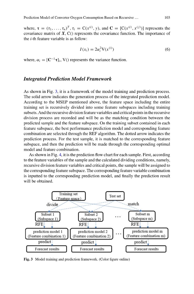
As shown in Fig. 3, it is a framework of the model training and prediction process.
The solid arrow indicates the generation process of the integrated prediction model.
According to the MSEP mentioned above, the feature space including the entire
training set is recursively divided into some feature subspaces including training
subsets. And the recursive division feature variables and critical points in the recursive
division process are recorded and will be as the matching condition between the
predicted sample and the feature subspace. On the training subset contained in each
feature subspace, the best performance prediction model and corresponding feature
combination are selected through the REF algorithm. The dotted arrow indicates the
prediction process. For the test sample, it is matched to the corresponding feature
subspace, and then the prediction will be made through the corresponding optimal
model and feature combination.
As shown in Fig. 4, it is the prediction flow chart for each sample. First, according
to the feature variables of the sample and the calculated dividing conditions, namely,
recursive division feature variables and critical points, the sample will be assigned to
the corresponding feature subspace. The corresponding feature variable combination
is inputted to the corresponding prediction model, and finally the prediction result
will be obtained.
Fig. 3 Model training and prediction framework. (Color figure online)
103
where, τ = (τ 1 , . . . , τ n )
T
, τ i = C(x
(i)
, y), and C = [C(x
(i)
, x
( j)
)] represents the
covariance matrix of X, C() represents the covariance function. The importance of
the i-th feature variable is as follow:
I (x i ) = 2α
2
i V(x
(i)
)
(6)
where, α i = [C
−1
τ] i , V() represents the variance function.
Integrated Prediction Model Framework
As shown in Fig. 3, it is a framework of the model training and prediction process.
The solid arrow indicates the generation process of the integrated prediction model.
According to the MSEP mentioned above, the feature space including the entire
training set is recursively divided into some feature subspaces including training
subsets. And the recursive division feature variables and critical points in the recursive
division process are recorded and will be as the matching condition between the
predicted sample and the feature subspace. On the training subset contained in each
feature subspace, the best performance prediction model and corresponding feature
combination are selected through the REF algorithm. The dotted arrow indicates the
prediction process. For the test sample, it is matched to the corresponding feature
subspace, and then the prediction will be made through the corresponding optimal
model and feature combination.
As shown in Fig. 4, it is the prediction flow chart for each sample. First, according
to the feature variables of the sample and the calculated dividing conditions, namely,
recursive division feature variables and critical points, the sample will be assigned to
the corresponding feature subspace. The corresponding feature variable combination
is inputted to the corresponding prediction model, and finally the prediction result
will be obtained.
Fig. 3 Model training and prediction framework. (Color figure online)