

For example, in the case of
119 Sn, there is a useful M 1 ½ ! 3/2 ! ½ transition
where the excited state has a lifetime of 26 ns (Fig. 9.19) [455], for which the
perturbation factor is:
G 22 t
ð Þ ¼
1
5
þ
4
5
Á cos ωt
ð Þ:
ð9:26Þ
and the angular frequency ω corresponds to ω ¼ ΔE/η ¼ eQ e V zz /2.
A slightly more complicated pattern occurs for
61 Ni SRPAC, where the excitations are M 1 3/2 ! 5/2 ! 3/2 transitions. For a Zeeman-split excited state with
magnetic field B and nuclear g-factor g, a random magnetic orientation and Larmor
frequency ω B ¼ À gμ N B/ħ, where μ N is the nuclear magneton, the perturbation
factor is given by:
G 22 t
ð Þ ¼
1
5
1 þ 2 cos ω B t þ 2 cos 2ω B t
ð
Þ
ð 9:27Þ
Although there are now two beat frequencies, there is still a tremendous simplification over the NFS experiment which involves beating between 12 different
frequencies. An example is shown later in Fig. 9.21.
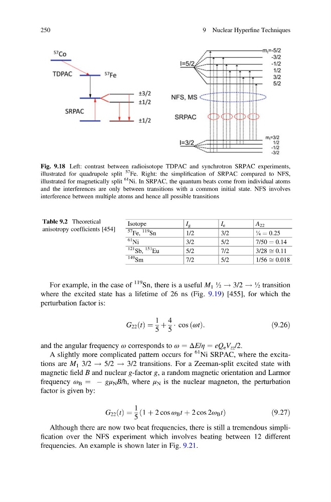
Fig. 9.18 Left: contrast between radioisotope TDPAC and synchrotron SRPAC experiments,
illustrated for quadrupole split
57
Fe. Right: the simplification of SRPAC compared to NFS,
illustrated for magnetically split
61
Ni. In SRPAC, the quantum beats come from individual atoms
and the interferences are only between transitions with a common initial state. NFS involves
interference between multiple atoms and hence all possible transitions
Table 9.2 Theoretical
anisotropy coefficients [454]
Isotope
I g
I e
A 22
57
Fe,
119
Sn
1/2
3/2
¼ ¼ 0.25
61
Ni
3/2
5/2
7/50 ¼ 0.14
121
Sb,
151 Eu
5/2
7/2
3/28 ffi 0.11
149
Sm
7/2
5/2
1/56 ffi 0.018
250
9 Nuclear Hyperfine Techniques
119 Sn, there is a useful M 1 ½ ! 3/2 ! ½ transition
where the excited state has a lifetime of 26 ns (Fig. 9.19) [455], for which the
perturbation factor is:
G 22 t
ð Þ ¼
1
5
þ
4
5
Á cos ωt
ð Þ:
ð9:26Þ
and the angular frequency ω corresponds to ω ¼ ΔE/η ¼ eQ e V zz /2.
A slightly more complicated pattern occurs for
61 Ni SRPAC, where the excitations are M 1 3/2 ! 5/2 ! 3/2 transitions. For a Zeeman-split excited state with
magnetic field B and nuclear g-factor g, a random magnetic orientation and Larmor
frequency ω B ¼ À gμ N B/ħ, where μ N is the nuclear magneton, the perturbation
factor is given by:
G 22 t
ð Þ ¼
1
5
1 þ 2 cos ω B t þ 2 cos 2ω B t
ð
Þ
ð 9:27Þ
Although there are now two beat frequencies, there is still a tremendous simplification over the NFS experiment which involves beating between 12 different
frequencies. An example is shown later in Fig. 9.21.
Fig. 9.18 Left: contrast between radioisotope TDPAC and synchrotron SRPAC experiments,
illustrated for quadrupole split
57
Fe. Right: the simplification of SRPAC compared to NFS,
illustrated for magnetically split
61
Ni. In SRPAC, the quantum beats come from individual atoms
and the interferences are only between transitions with a common initial state. NFS involves
interference between multiple atoms and hence all possible transitions
Table 9.2 Theoretical
anisotropy coefficients [454]
Isotope
I g
I e
A 22
57
Fe,
119
Sn
1/2
3/2
¼ ¼ 0.25
61
Ni
3/2
5/2
7/50 ¼ 0.14
121
Sb,
151 Eu
5/2
7/2
3/28 ffi 0.11
149
Sm
7/2
5/2
1/56 ffi 0.018
250
9 Nuclear Hyperfine Techniques