

multiplet features in the final state are similar to those discussed earlier with respect
to transition metal L- and lanthanide M-edges (Chap. 7). The strongest effects are
seen with the largest number of unpaired valence electrons, such as d
5 Mn(II) or f
7
Gd(III).
As an example, consider Mn Kβ fluorescence, and compare it to Mn Kα fluorescence (Fig. 8.4). For Mn(II), in atomic nomenclature, the two allowed terms for the
“initial” 1s
1 3d
5 configuration are
7 S and
5 S. Kβ fluorescence involves filling the 1s
vacancy from the 3p shell, so the final configuration is 3p
5 3d
5 , which yields two final
terms:
7 P and
5
P. What is different now, compared to the Kα case, is the strength of
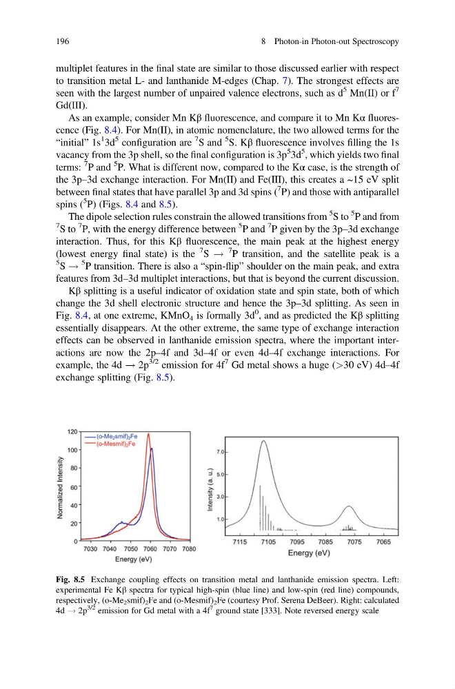
the 3p–3d exchange interaction. For Mn(II) and Fe(III), this creates a ~15 eV split
between final states that have parallel 3p and 3d spins (
7 P) and those with antiparallel
spins (
5
P) (Figs. 8.4 and 8.5).
The dipole selection rules constrain the allowed transitions from
5 S to
5 P and from
7 S to
7 P, with the energy difference between
5 P and
7 P given by the 3p–3d exchange
interaction. Thus, for this Kβ fluorescence, the main peak at the highest energy
(lowest energy final state) is the
7 S !
7 P transition, and the satellite peak is a
5 S !
5 P transition. There is also a “spin-flip” shoulder on the main peak, and extra
features from 3d–3d multiplet interactions, but that is beyond the current discussion.
Kβ splitting is a useful indicator of oxidation state and spin state, both of which
change the 3d shell electronic structure and hence the 3p–3d splitting. As seen in
Fig. 8.4, at one extreme, KMnO 4 is formally 3d
0 , and as predicted the Kβ splitting
essentially disappears. At the other extreme, the same type of exchange interaction
effects can be observed in lanthanide emission spectra, where the important interactions are now the 2p–4f and 3d–4f or even 4d–4f exchange interactions. For
example, the 4d ! 2p
3/2 emission for 4f
7 Gd metal shows a huge (>30 eV) 4d–4f
exchange splitting (Fig. 8.5).
Fig. 8.5 Exchange coupling effects on transition metal and lanthanide emission spectra. Left:
experimental Fe Kβ spectra for typical high-spin (blue line) and low-spin (red line) compounds,
respectively, (o-Me 2 smif) 2 Fe and (o-Mesmif) 2 Fe (courtesy Prof. Serena DeBeer). Right: calculated
4d ! 2p
3/2 emission for Gd metal with a 4f
7 ground state [333]. Note reversed energy scale
196
8 Photon-in Photon-out Spectroscopy
to transition metal L- and lanthanide M-edges (Chap. 7). The strongest effects are
seen with the largest number of unpaired valence electrons, such as d
5 Mn(II) or f
7
Gd(III).
As an example, consider Mn Kβ fluorescence, and compare it to Mn Kα fluorescence (Fig. 8.4). For Mn(II), in atomic nomenclature, the two allowed terms for the
“initial” 1s
1 3d
5 configuration are
7 S and
5 S. Kβ fluorescence involves filling the 1s
vacancy from the 3p shell, so the final configuration is 3p
5 3d
5 , which yields two final
terms:
7 P and
5
P. What is different now, compared to the Kα case, is the strength of
the 3p–3d exchange interaction. For Mn(II) and Fe(III), this creates a ~15 eV split
between final states that have parallel 3p and 3d spins (
7 P) and those with antiparallel
spins (
5
P) (Figs. 8.4 and 8.5).
The dipole selection rules constrain the allowed transitions from
5 S to
5 P and from
7 S to
7 P, with the energy difference between
5 P and
7 P given by the 3p–3d exchange
interaction. Thus, for this Kβ fluorescence, the main peak at the highest energy
(lowest energy final state) is the
7 S !
7 P transition, and the satellite peak is a
5 S !
5 P transition. There is also a “spin-flip” shoulder on the main peak, and extra
features from 3d–3d multiplet interactions, but that is beyond the current discussion.
Kβ splitting is a useful indicator of oxidation state and spin state, both of which
change the 3d shell electronic structure and hence the 3p–3d splitting. As seen in
Fig. 8.4, at one extreme, KMnO 4 is formally 3d
0 , and as predicted the Kβ splitting
essentially disappears. At the other extreme, the same type of exchange interaction
effects can be observed in lanthanide emission spectra, where the important interactions are now the 2p–4f and 3d–4f or even 4d–4f exchange interactions. For
example, the 4d ! 2p
3/2 emission for 4f
7 Gd metal shows a huge (>30 eV) 4d–4f
exchange splitting (Fig. 8.5).
Fig. 8.5 Exchange coupling effects on transition metal and lanthanide emission spectra. Left:
experimental Fe Kβ spectra for typical high-spin (blue line) and low-spin (red line) compounds,
respectively, (o-Me 2 smif) 2 Fe and (o-Mesmif) 2 Fe (courtesy Prof. Serena DeBeer). Right: calculated
4d ! 2p
3/2 emission for Gd metal with a 4f
7 ground state [333]. Note reversed energy scale
196
8 Photon-in Photon-out Spectroscopy