

multiplet theory (“CTMT”) [285]. These models describe the final states as atomic
multiplets that are perturbed by the ligand field of the surrounding atoms. CTMT
begins by evaluating the atomic multiplets that arise from a given configuration of
core hole and valence electrons. Symmetry and ligand field parameters are then used
to calculate how these multiplets are split by the ligand environment. For those who
care about the origins of this theory [286,287], there are key papers by Thole,
Sawatzky, van der Laan and coworkers [288], who built on group theory by Butler
[289] and atomic Hartree-Fock methods from Cowan and coworkers [290].
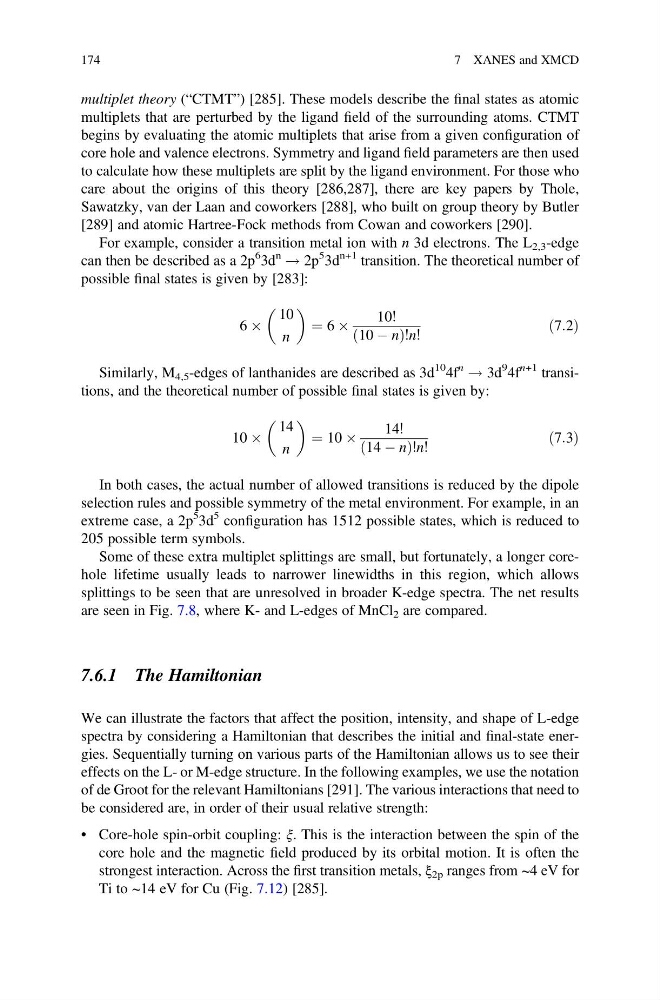
For example, consider a transition metal ion with n 3d electrons. The L 2,3 -edge
can then be described as a 2p
6 3d
n
! 2p
5 3d
n+1 transition. The theoretical number of
possible final states is given by [283]:
6 Â
10
n
¼ 6 Â
10!
10 À n
ð
Þ!n!
ð7:2Þ
Similarly, M 4,5 -edges of lanthanides are described as 3d
10 4f
n
! 3d
9 4f
n+1 transitions, and the theoretical number of possible final states is given by:
10 Â
14
n
¼ 10 Â
14!
14 À n
ð
Þ!n!
ð7:3Þ
In both cases, the actual number of allowed transitions is reduced by the dipole
selection rules and possible symmetry of the metal environment. For example, in an
extreme case, a 2p
5 3d
5 configuration has 1512 possible states, which is reduced to
205 possible term symbols.
Some of these extra multiplet splittings are small, but fortunately, a longer corehole lifetime usually leads to narrower linewidths in this region, which allows
splittings to be seen that are unresolved in broader K-edge spectra. The net results
are seen in Fig. 7.8, where K- and L-edges of MnCl 2 are compared.
7.6.1 The Hamiltonian
We can illustrate the factors that affect the position, intensity, and shape of L-edge
spectra by considering a Hamiltonian that describes the initial and final-state energies. Sequentially turning on various parts of the Hamiltonian allows us to see their
effects on the L- or M-edge structure. In the following examples, we use the notation
of de Groot for the relevant Hamiltonians [291]. The various interactions that need to
be considered are, in order of their usual relative strength:
• Core-hole spin-orbit coupling: ξ. This is the interaction between the spin of the
core hole and the magnetic field produced by its orbital motion. It is often the
strongest interaction. Across the first transition metals, ξ 2p ranges from ~4 eV for
Ti to ~14 eV for Cu (Fig. 7.12) [285].
174
7 XANES and XMCD
multiplets that are perturbed by the ligand field of the surrounding atoms. CTMT
begins by evaluating the atomic multiplets that arise from a given configuration of
core hole and valence electrons. Symmetry and ligand field parameters are then used
to calculate how these multiplets are split by the ligand environment. For those who
care about the origins of this theory [286,287], there are key papers by Thole,
Sawatzky, van der Laan and coworkers [288], who built on group theory by Butler
[289] and atomic Hartree-Fock methods from Cowan and coworkers [290].
For example, consider a transition metal ion with n 3d electrons. The L 2,3 -edge
can then be described as a 2p
6 3d
n
! 2p
5 3d
n+1 transition. The theoretical number of
possible final states is given by [283]:
6 Â
10
n
¼ 6 Â
10!
10 À n
ð
Þ!n!
ð7:2Þ
Similarly, M 4,5 -edges of lanthanides are described as 3d
10 4f
n
! 3d
9 4f
n+1 transitions, and the theoretical number of possible final states is given by:
10 Â
14
n
¼ 10 Â
14!
14 À n
ð
Þ!n!
ð7:3Þ
In both cases, the actual number of allowed transitions is reduced by the dipole
selection rules and possible symmetry of the metal environment. For example, in an
extreme case, a 2p
5 3d
5 configuration has 1512 possible states, which is reduced to
205 possible term symbols.
Some of these extra multiplet splittings are small, but fortunately, a longer corehole lifetime usually leads to narrower linewidths in this region, which allows
splittings to be seen that are unresolved in broader K-edge spectra. The net results
are seen in Fig. 7.8, where K- and L-edges of MnCl 2 are compared.
7.6.1 The Hamiltonian
We can illustrate the factors that affect the position, intensity, and shape of L-edge
spectra by considering a Hamiltonian that describes the initial and final-state energies. Sequentially turning on various parts of the Hamiltonian allows us to see their
effects on the L- or M-edge structure. In the following examples, we use the notation
of de Groot for the relevant Hamiltonians [291]. The various interactions that need to
be considered are, in order of their usual relative strength:
• Core-hole spin-orbit coupling: ξ. This is the interaction between the spin of the
core hole and the magnetic field produced by its orbital motion. It is often the
strongest interaction. Across the first transition metals, ξ 2p ranges from ~4 eV for
Ti to ~14 eV for Cu (Fig. 7.12) [285].
174
7 XANES and XMCD