

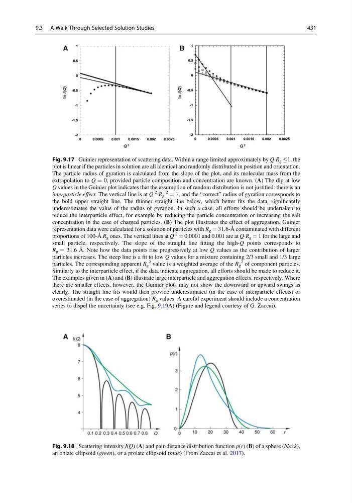
Fig. 9.17 Guinier representation of scattering data. Within a range limited approximately by QÁR g 1, the
plot is linear if the particles in solution are all identical and randomly distributed in position and orientation.
The particle radius of gyration is calculated from the slope of the plot, and its molecular mass from the
extrapolation to Q ¼ 0, provided particle composition and concentration are known. (A) The dip at low
Q values in the Guinier plot indicates that the assumption of random distribution is not justified: there is an
interparticle effect. The vertical line is at Q
2
ÁR g
2 ¼ 1, and the “correct” radius of gyration corresponds to
the bold upper straight line. The thinner straight line below, which better fits the data, significantly
underestimates the value of the radius of gyration. In such a case, all efforts should be undertaken to
reduce the interparticle effect, for example by reducing the particle concentration or increasing the salt
concentration in the case of charged particles. (B) The plot illustrates the effect of aggregation. Guinier
representation data were calculated for a solution of particles with R g ¼ 31.6-Å contaminated with different
proportions of 100-Å R g ones. The vertical lines at Q
2 ¼ 0.0001 and 0.001 are at QÁR g ¼ 1 for the large and
small particle, respectively. The slope of the straight line fitting the high-Q points corresponds to
R g ¼ 31.6 Å. Note how the data points rise progressively at low Q values as the contribution of larger
particles increases. The steep line is a fit to low Q values for a mixture containing 2/3 small and 1/3 large
particles. The corresponding apparent R g
2 value is a weighted average of the R g
2 of component particles.
Similarly to the interparticle effect, if the data indicate aggregation, all efforts should be made to reduce it.
The examples given in (A) and (B) illustrate large interparticle and aggregation effects, respectively. Where
there are smaller effects, however, the Guinier plots may not show the downward or upward swings as
clearly. The straight line fits would then provide underestimated (in the case of interparticle effects) or
overestimated (in the case of aggregation) R g values. A careful experiment should include a concentration
series to dispel the uncertainty (see e.g. Fig. 9.19A) (Figure and legend courtesy of G. Zaccai).
Fig. 9.18 Scattering intensity I(Q) (A) and pair-distance distribution function p(r) (B) of a sphere (black),
an oblate ellipsoid (green), or a prolate ellipsoid (blue) (From Zaccai et al. 2017).
9.3 A Walk Through Selected Solution Studies
431
plot is linear if the particles in solution are all identical and randomly distributed in position and orientation.
The particle radius of gyration is calculated from the slope of the plot, and its molecular mass from the
extrapolation to Q ¼ 0, provided particle composition and concentration are known. (A) The dip at low
Q values in the Guinier plot indicates that the assumption of random distribution is not justified: there is an
interparticle effect. The vertical line is at Q
2
ÁR g
2 ¼ 1, and the “correct” radius of gyration corresponds to
the bold upper straight line. The thinner straight line below, which better fits the data, significantly
underestimates the value of the radius of gyration. In such a case, all efforts should be undertaken to
reduce the interparticle effect, for example by reducing the particle concentration or increasing the salt
concentration in the case of charged particles. (B) The plot illustrates the effect of aggregation. Guinier
representation data were calculated for a solution of particles with R g ¼ 31.6-Å contaminated with different
proportions of 100-Å R g ones. The vertical lines at Q
2 ¼ 0.0001 and 0.001 are at QÁR g ¼ 1 for the large and
small particle, respectively. The slope of the straight line fitting the high-Q points corresponds to
R g ¼ 31.6 Å. Note how the data points rise progressively at low Q values as the contribution of larger
particles increases. The steep line is a fit to low Q values for a mixture containing 2/3 small and 1/3 large
particles. The corresponding apparent R g
2 value is a weighted average of the R g
2 of component particles.
Similarly to the interparticle effect, if the data indicate aggregation, all efforts should be made to reduce it.
The examples given in (A) and (B) illustrate large interparticle and aggregation effects, respectively. Where
there are smaller effects, however, the Guinier plots may not show the downward or upward swings as
clearly. The straight line fits would then provide underestimated (in the case of interparticle effects) or
overestimated (in the case of aggregation) R g values. A careful experiment should include a concentration
series to dispel the uncertainty (see e.g. Fig. 9.19A) (Figure and legend courtesy of G. Zaccai).
Fig. 9.18 Scattering intensity I(Q) (A) and pair-distance distribution function p(r) (B) of a sphere (black),
an oblate ellipsoid (green), or a prolate ellipsoid (blue) (From Zaccai et al. 2017).
9.3 A Walk Through Selected Solution Studies
431