

4.6.5.2 Polymer Composition (Microstructure)
Because the physical-chemical properties of a polymer are closely linked to its microstructure (or composition) (Liu et al.
2007), the distribution of the different comonomers along the polymer’s backbone (see Fig. 4.44) must be known, and
controlled as much as possible. Indeed, the physical properties of the final polymers may turn out to be very different
from those expected if this parameter is not properly mastered. This problem has been identified quite early and
characterized for RP during the first half of the twentieth century (Mayo and Lewis 1944; Lewis et al. 1948). For a
given copolymer in formation, the evolution of the concentration of the two monomers M 1 and M 2 is given by:
d M 1
½
d M 2
½
¼
M 1
½
M 2
½
∙
r 1 M 1
½ þ M 2
½
M 1
½ þr 2 M 2
½
ð4:28Þ
where [M 1 ] and [M 2 ] are the concentrations of unreacted monomers, r 1 is the ratio of the rate constants for the reaction of
an M 1 -type radical with M 1 and M 2 , respectively, and r 2 is the ratio for reaction of an M 2 -type radical with M 2 and M 1 ,
respectively.
By introducing f and F, the molar fractions of monomer in the feed and in the copolymer, respectively, Eq. 4.28
becomes:
F 1 ¼ 1 À F 2 ¼
d M 1
½
d M 1
½ þd M 2
½
¼
r 1 f
2
1 þ f 1 f 2
r 1 f
2
1 þ 2f 1 f 2 þ r 2 f
2
2
ð4:29Þ
hF 1 i, the cumulative value of F 1 (i.e. the average value of the molar fraction of M 1 that has been incorporated into the
various terminated and growing macromolecular chains formed since the initiation), may be expressed as:
F 1
h i ¼
f 1, 0 À f 1, t 1 À α
ð
Þ
α
ð4:30Þ
where f 1,0 and f 1,t are initial and instantaneous value of f 1 , respectively, and α is as defined in Eq. 4.23.
Although Eqs. 4.28 and 4.29 were established in the context of RP, they are valid for all kinds of polymerization.
Various rearrangements of Eq. 4.29 (not shown) have been proposed to deduce the value of r 1 and r 2 (Alfrey and Price
1947; Lewis et al. 1948; Fineman and Ross 1950; Kelen et al. 1980).
F and f are accessible by FTIR (Parambil et al. 2012), NMR (Bataille and Bourassa 1989; Cracowski et al. 2010;
Parambil et al. 2012), or elemental analyses (Cracowski et al. 2010) of the feed and of the copolymer.
Five different cases are commonly considered:
• r 1 % r 2 % 1: generated radicals react randomly with both monomers, and the relative rates of monomer
consumption are determined only by the relative monomer concentrations in the feed mixture. The composition of monomers in the copolymer is approximately identical to that in the feed, and the distribution of each
monomer is expected to be random. Equation 4.28 becomes:
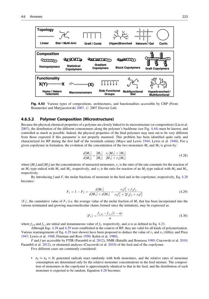
Fig. 4.43 Various types of compositions, architectures, and functionalities accessible by CRP (From
Braunecker and Matyjasziewski 2007, # 2007 Elsevier Ltd).
4.6 Annexes
223
Because the physical-chemical properties of a polymer are closely linked to its microstructure (or composition) (Liu et al.
2007), the distribution of the different comonomers along the polymer’s backbone (see Fig. 4.44) must be known, and
controlled as much as possible. Indeed, the physical properties of the final polymers may turn out to be very different
from those expected if this parameter is not properly mastered. This problem has been identified quite early and
characterized for RP during the first half of the twentieth century (Mayo and Lewis 1944; Lewis et al. 1948). For a
given copolymer in formation, the evolution of the concentration of the two monomers M 1 and M 2 is given by:
d M 1
½
d M 2
½
¼
M 1
½
M 2
½
∙
r 1 M 1
½ þ M 2
½
M 1
½ þr 2 M 2
½
ð4:28Þ
where [M 1 ] and [M 2 ] are the concentrations of unreacted monomers, r 1 is the ratio of the rate constants for the reaction of
an M 1 -type radical with M 1 and M 2 , respectively, and r 2 is the ratio for reaction of an M 2 -type radical with M 2 and M 1 ,
respectively.
By introducing f and F, the molar fractions of monomer in the feed and in the copolymer, respectively, Eq. 4.28
becomes:
F 1 ¼ 1 À F 2 ¼
d M 1
½
d M 1
½ þd M 2
½
¼
r 1 f
2
1 þ f 1 f 2
r 1 f
2
1 þ 2f 1 f 2 þ r 2 f
2
2
ð4:29Þ
hF 1 i, the cumulative value of F 1 (i.e. the average value of the molar fraction of M 1 that has been incorporated into the
various terminated and growing macromolecular chains formed since the initiation), may be expressed as:
F 1
h i ¼
f 1, 0 À f 1, t 1 À α
ð
Þ
α
ð4:30Þ
where f 1,0 and f 1,t are initial and instantaneous value of f 1 , respectively, and α is as defined in Eq. 4.23.
Although Eqs. 4.28 and 4.29 were established in the context of RP, they are valid for all kinds of polymerization.
Various rearrangements of Eq. 4.29 (not shown) have been proposed to deduce the value of r 1 and r 2 (Alfrey and Price
1947; Lewis et al. 1948; Fineman and Ross 1950; Kelen et al. 1980).
F and f are accessible by FTIR (Parambil et al. 2012), NMR (Bataille and Bourassa 1989; Cracowski et al. 2010;
Parambil et al. 2012), or elemental analyses (Cracowski et al. 2010) of the feed and of the copolymer.
Five different cases are commonly considered:
• r 1 % r 2 % 1: generated radicals react randomly with both monomers, and the relative rates of monomer
consumption are determined only by the relative monomer concentrations in the feed mixture. The composition of monomers in the copolymer is approximately identical to that in the feed, and the distribution of each
monomer is expected to be random. Equation 4.28 becomes:
Fig. 4.43 Various types of compositions, architectures, and functionalities accessible by CRP (From
Braunecker and Matyjasziewski 2007, # 2007 Elsevier Ltd).
4.6 Annexes
223