

338
M. Springborg et al.
18.2.3 The SCF Equations for the Infinite Periodic System
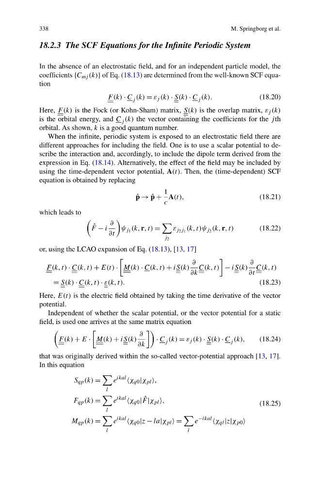
In the absence of an electrostatic field, and for an independent particle model, the
coefficients {C mj (k)} of Eq. (18.13) are determined from the well-known SCF equation
F (k) · C j (k) = ε j (k) · S(k) · C j (k).
(18.20)
Here, F (k) is the Fock (or Kohn-Sham) matrix, S(k) is the overlap matrix, ε j (k)
is the orbital energy, and C j (k) the vector containing the coefficients for the j th
orbital. As shown, k is a good quantum number.
When the infinite, periodic system is exposed to an electrostatic field there are
different approaches for including the field. One is to use a scalar potential to describe the interaction and, accordingly, to include the dipole term derived from the
expression in Eq. (18.14). Alternatively, the effect of the field may be included by
using the time-dependent vector potential, A(t). Then, the (time-dependent) SCF
equation is obtained by replacing
ˆ
p → ˆ
p +
1
c
A(t),
(18.21)
which leads to
ˆ
F − i
∂
∂t
ψ j 1 (k, r, t) =
j 2
ε j 2 j 1 (k, t)ψ j 2 (k, r, t)
(18.22)
or, using the LCAO expansion of Eq. (18.13), [13, 17]
F (k, t) · C(k, t) + E(t) ·
M(k) · C(k, t) + iS(k)
∂
∂k
C(k, t)
− iS(k)
∂
∂t
C(k, t)
= S(k) · C(k, t) · ε(k, t).
(18.23)
Here, E(t) is the electric field obtained by taking the time derivative of the vector
potential.
Independent of whether the scalar potential, or the vector potential for a static
field, is used one arrives at the same matrix equation
F (k) + E ·
M(k) + iS(k)
∂
∂k
· C j (k) = ε j (k) · S(k) · C j (k),
(18.24)
that was originally derived within the so-called vector-potential approach [13, 17].
In this equation
S qp (k) =
l
e
ikal
χ q0 |χ pl ,
F qp (k) =
l
e
ikal
χ q0 | ˆ
F |χ pl ,
M qp (k) =
l
e
ikal
χ q0 |z − la|χ pl =
l
e
−ikal
χ ql |z|χ p0
(18.25)
M. Springborg et al.
18.2.3 The SCF Equations for the Infinite Periodic System
In the absence of an electrostatic field, and for an independent particle model, the
coefficients {C mj (k)} of Eq. (18.13) are determined from the well-known SCF equation
F (k) · C j (k) = ε j (k) · S(k) · C j (k).
(18.20)
Here, F (k) is the Fock (or Kohn-Sham) matrix, S(k) is the overlap matrix, ε j (k)
is the orbital energy, and C j (k) the vector containing the coefficients for the j th
orbital. As shown, k is a good quantum number.
When the infinite, periodic system is exposed to an electrostatic field there are
different approaches for including the field. One is to use a scalar potential to describe the interaction and, accordingly, to include the dipole term derived from the
expression in Eq. (18.14). Alternatively, the effect of the field may be included by
using the time-dependent vector potential, A(t). Then, the (time-dependent) SCF
equation is obtained by replacing
ˆ
p → ˆ
p +
1
c
A(t),
(18.21)
which leads to
ˆ
F − i
∂
∂t
ψ j 1 (k, r, t) =
j 2
ε j 2 j 1 (k, t)ψ j 2 (k, r, t)
(18.22)
or, using the LCAO expansion of Eq. (18.13), [13, 17]
F (k, t) · C(k, t) + E(t) ·
M(k) · C(k, t) + iS(k)
∂
∂k
C(k, t)
− iS(k)
∂
∂t
C(k, t)
= S(k) · C(k, t) · ε(k, t).
(18.23)
Here, E(t) is the electric field obtained by taking the time derivative of the vector
potential.
Independent of whether the scalar potential, or the vector potential for a static
field, is used one arrives at the same matrix equation
F (k) + E ·
M(k) + iS(k)
∂
∂k
· C j (k) = ε j (k) · S(k) · C j (k),
(18.24)
that was originally derived within the so-called vector-potential approach [13, 17].
In this equation
S qp (k) =
l
e
ikal
χ q0 |χ pl ,
F qp (k) =
l
e
ikal
χ q0 | ˆ
F |χ pl ,
M qp (k) =
l
e
ikal
χ q0 |z − la|χ pl =
l
e
−ikal
χ ql |z|χ p0
(18.25)