

166
A.V. Glushkov
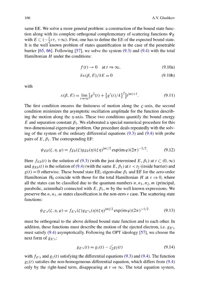
same EE. We solve a more general problem: a construction of the bound state function along with its complete orthogonal complementary of scattering functions Ψ E
with E ⊂ (−
1
2 ετ, +∞). First, one has to define the EE of the expected bound state.
It is the well known problem of states quantification in the case of the penetrable
barrier [65, 66]. Following [57], we solve the system (9.3) and (9.4) with the total
Hamiltonian H under the conditions:
f (t) → 0 at t ⇒ ∞,
(9.10a)
∂x(β, E)/∂E = 0
(9.10b)
with
x(β, E) = lim
t⇒∞
g
2 (t) +
g
(t)/k
2
t
|m|+1 .
(9.11)
The first condition ensures the finiteness of motion along the ς -axis, the second
condition minimizes the asymptotic oscillation amplitude for the function describing the motion along the η-axis. These two conditions quantify the bound energy
E and separation constant β 1 . We elaborated a special numerical procedure for this
two-dimensional eigenvalue problem. Our procedure deals repeatedly with the solving of the system of the ordinary differential equations (9.3) and (9.4) with probe
pairs of E, β 1 . The corresponding EF:
ψ Eb (ζ, η, ϕ) = f Eb (ζ )g Eb (η)(ζ η)
|m|/2 exp(im ϕ)(2π)
−1/2 .
(9.12)
Here f Eb (t) is the solution of (9.3) (with the just determined E, β 1 ) at t ⊂ (0, ∞)
and g Eb (t) is the solution of (9.4) (with the same E, β 1 ) at t < t 2 (inside barrier) and
g(t) = 0 otherwise. These bound state EE, eigenvalue β 1 and EF for the zero-order
Hamiltonian H 0 coincide with those for the total Hamiltonian H at ε ⇒ 0, where
all the states can be classified due to the quantum numbers n, n 1 , n 2 , m (principal,
parabolic, azimuthal) connected with E, β 1 , m by the well known expressions. We
preserve the n, n 1 , m states classification in the non-zero ε case. The scattering state
functions:
ψ E s (ζ, η, ϕ) = f E s (ζ )g E s (η)(ζ η)
|m|/2 exp(im ϕ)(2π)
−1/2
(9.13)
must be orthogonal to the above defined bound state function and to each other. In
addition, these functions must describe the motion of the ejected electron, i.e. g E s
must satisfy (9.4) asymptotically. Following the OPT ideology [57], we choose the
next form of g E s :
g E s (t) = g 1 (t) − z
2 g 2 (t)
(9.14)
with f E s and g 1 (t) satisfying the differential equations (9.3) and (9.4). The function
g 2 (t) satisfies the non-homogeneous differential equation, which differs from (9.4)
only by the right-hand term, disappearing at t ⇒ ∞. The total equation system,
A.V. Glushkov
same EE. We solve a more general problem: a construction of the bound state function along with its complete orthogonal complementary of scattering functions Ψ E
with E ⊂ (−
1
2 ετ, +∞). First, one has to define the EE of the expected bound state.
It is the well known problem of states quantification in the case of the penetrable
barrier [65, 66]. Following [57], we solve the system (9.3) and (9.4) with the total
Hamiltonian H under the conditions:
f (t) → 0 at t ⇒ ∞,
(9.10a)
∂x(β, E)/∂E = 0
(9.10b)
with
x(β, E) = lim
t⇒∞
g
2 (t) +
g
(t)/k
2
t
|m|+1 .
(9.11)
The first condition ensures the finiteness of motion along the ς -axis, the second
condition minimizes the asymptotic oscillation amplitude for the function describing the motion along the η-axis. These two conditions quantify the bound energy
E and separation constant β 1 . We elaborated a special numerical procedure for this
two-dimensional eigenvalue problem. Our procedure deals repeatedly with the solving of the system of the ordinary differential equations (9.3) and (9.4) with probe
pairs of E, β 1 . The corresponding EF:
ψ Eb (ζ, η, ϕ) = f Eb (ζ )g Eb (η)(ζ η)
|m|/2 exp(im ϕ)(2π)
−1/2 .
(9.12)
Here f Eb (t) is the solution of (9.3) (with the just determined E, β 1 ) at t ⊂ (0, ∞)
and g Eb (t) is the solution of (9.4) (with the same E, β 1 ) at t < t 2 (inside barrier) and
g(t) = 0 otherwise. These bound state EE, eigenvalue β 1 and EF for the zero-order
Hamiltonian H 0 coincide with those for the total Hamiltonian H at ε ⇒ 0, where
all the states can be classified due to the quantum numbers n, n 1 , n 2 , m (principal,
parabolic, azimuthal) connected with E, β 1 , m by the well known expressions. We
preserve the n, n 1 , m states classification in the non-zero ε case. The scattering state
functions:
ψ E s (ζ, η, ϕ) = f E s (ζ )g E s (η)(ζ η)
|m|/2 exp(im ϕ)(2π)
−1/2
(9.13)
must be orthogonal to the above defined bound state function and to each other. In
addition, these functions must describe the motion of the ejected electron, i.e. g E s
must satisfy (9.4) asymptotically. Following the OPT ideology [57], we choose the
next form of g E s :
g E s (t) = g 1 (t) − z
2 g 2 (t)
(9.14)
with f E s and g 1 (t) satisfying the differential equations (9.3) and (9.4). The function
g 2 (t) satisfies the non-homogeneous differential equation, which differs from (9.4)
only by the right-hand term, disappearing at t ⇒ ∞. The total equation system,