

114
S.O. Adamson et al.
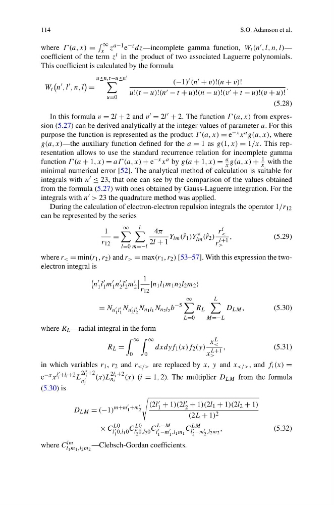
where Γ (a, x) =
∞
x z a−1 e −z dz—incomplete gamma function, W t (n , l, n, l)—
coefficient of the term z t in the product of two associated Laguerre polynomials.
This coefficient is calculated by the formula
W t
n
, l
, n, l
=
u≤n,t−u≤n
u=0
(−1) t (n + v)!(n + v)!
u!(t − u)!(n − t + u)!(n − u)!(v + t − u)!(v + u)!
.
(5.28)
In this formula v = 2l + 2 and v = 2l + 2. The function Γ (a, x) from expression (5.27) can be derived analytically at the integer values of parameter a. For this
purpose the function is represented as the product Γ (a, x) = e −x x a g(a, x), where
g(a, x)—the auxiliary function defined for the a = 1 as g(1, x) = 1/x. This representation allows to use the standard recurrence relation for incomplete gamma
function Γ (a + 1, x) = aΓ (a, x) + e −x x a by g(a + 1, x) =
a
x g(a, x) +
1
x with the
minimal numerical error [52]. The analytical method of calculation is suitable for
integrals with n ≤ 23, that one can see by the comparison of the values obtained
from the formula (5.27) with ones obtained by Gauss-Laguerre integration. For the
integrals with n > 23 the quadrature method was applied.
During the calculation of electron-electron repulsion integrals the operator 1/r 12
can be represented by the series
1
r 12
=
∞
l=0
l
m=−l
4π
2l + 1
Y lm (ˆ r 1 )Y
∗
lm (ˆ r 2 )
r l
<
r
l+1
>
,
(5.29)
where r < = min(r 1 , r 2 ) and r > = max(r 1 , r 2 ) [53–57]. With this expression the twoelectron integral is
n
1 l
1 m
1 n
2 l
2 m
2
1
r 12
|n 1 l 1 m 1 n 2 l 2 m 2
= N n
1 l
1
N n
2 l
2
N n 1 l 1 N n 2 l 2 b
−5
∞
L=0
R L
L
M=−L
D LM ,
(5.30)
where R L —radial integral in the form
R L =
∞
0
∞
0
dxdyf 1 (x)f 2 (y)
x L
<
x
L+1
>
,
(5.31)
in which variables r 1 , r 2 and r are replaced by x, y and x , and f i (x) =
e −x x
l
i +l i +2 L
2l
i +2
n
i
(x)L
2l i +2
n i
(x) (i = 1, 2). The multiplier D LM from the formula
(5.30) is
D LM = (−1)
m+m
1 +m
2
(2l
1 + 1)(2l
2 + 1)(2l 1 + 1)(2l 2 + 1)
(2L + 1) 2
× C
L0
l
1 0,l 1 0
C
L0
l
2 0,l 2 0
C
L−M
l
1 −m
1 ,l 1 m 1
C
LM
l
2 −m
2 ,l 2 m 2
,
(5.32)
where C lm
l 1 m 1 ,l 2 m 2
—Clebsch-Gordan coefficients.
S.O. Adamson et al.
where Γ (a, x) =
∞
x z a−1 e −z dz—incomplete gamma function, W t (n , l, n, l)—
coefficient of the term z t in the product of two associated Laguerre polynomials.
This coefficient is calculated by the formula
W t
n
, l
, n, l
=
u≤n,t−u≤n
u=0
(−1) t (n + v)!(n + v)!
u!(t − u)!(n − t + u)!(n − u)!(v + t − u)!(v + u)!
.
(5.28)
In this formula v = 2l + 2 and v = 2l + 2. The function Γ (a, x) from expression (5.27) can be derived analytically at the integer values of parameter a. For this
purpose the function is represented as the product Γ (a, x) = e −x x a g(a, x), where
g(a, x)—the auxiliary function defined for the a = 1 as g(1, x) = 1/x. This representation allows to use the standard recurrence relation for incomplete gamma
function Γ (a + 1, x) = aΓ (a, x) + e −x x a by g(a + 1, x) =
a
x g(a, x) +
1
x with the
minimal numerical error [52]. The analytical method of calculation is suitable for
integrals with n ≤ 23, that one can see by the comparison of the values obtained
from the formula (5.27) with ones obtained by Gauss-Laguerre integration. For the
integrals with n > 23 the quadrature method was applied.
During the calculation of electron-electron repulsion integrals the operator 1/r 12
can be represented by the series
1
r 12
=
∞
l=0
l
m=−l
4π
2l + 1
Y lm (ˆ r 1 )Y
∗
lm (ˆ r 2 )
r l
<
r
l+1
>
,
(5.29)
where r < = min(r 1 , r 2 ) and r > = max(r 1 , r 2 ) [53–57]. With this expression the twoelectron integral is
n
1 l
1 m
1 n
2 l
2 m
2
1
r 12
|n 1 l 1 m 1 n 2 l 2 m 2
= N n
1 l
1
N n
2 l
2
N n 1 l 1 N n 2 l 2 b
−5
∞
L=0
R L
L
M=−L
D LM ,
(5.30)
where R L —radial integral in the form
R L =
∞
0
∞
0
dxdyf 1 (x)f 2 (y)
x L
<
x
L+1
>
,
(5.31)
in which variables r 1 , r 2 and r are replaced by x, y and x , and f i (x) =
e −x x
l
i +l i +2 L
2l
i +2
n
i
(x)L
2l i +2
n i
(x) (i = 1, 2). The multiplier D LM from the formula
(5.30) is
D LM = (−1)
m+m
1 +m
2
(2l
1 + 1)(2l
2 + 1)(2l 1 + 1)(2l 2 + 1)
(2L + 1) 2
× C
L0
l
1 0,l 1 0
C
L0
l
2 0,l 2 0
C
L−M
l
1 −m
1 ,l 1 m 1
C
LM
l
2 −m
2 ,l 2 m 2
,
(5.32)
where C lm
l 1 m 1 ,l 2 m 2
—Clebsch-Gordan coefficients.