

92
E.J. Brändas
where the energy (anticommutator) superoperator, see Prigogine [22], is equipped
with a complex conjugate sign in the bra-position. The latter is a necessity in order
to analytically continue the resonance solution into the complex plane, for more
details see Ref. [15]. Writing the Hamiltonian as a sum of two-body operators the
total energy follows from a simple trace formula. The formal solution of Eq. (4.15)
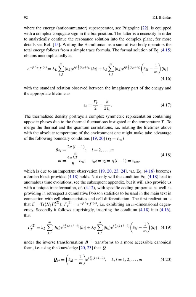
obtains uncomplicatedly as
e
−β ˆ
L B Γ
(2)
= λ L
m
k,l
|h k e
iβ
1
2 (ε k +ε l )
h l | + λ S
m
k,l
|h k e
iβ
1
2 (ε k +ε l )
δ kl −
1
m
h l |
(4.16)
with the standard relation observed between the imaginary part of the energy and
the appropriate lifetime as
ε k =
Γ k
2
=
2τ k
.
(4.17)
The thermalized density portrays a complex symmetric representation containing
apposite phases due to the thermal fluctuations instigated at the temperature T . To
merge the thermal and the quantum correlations, i.e. relating the lifetimes above
with the absolute temperature of the environment one might make take advantage
of the following boundary conditions [19, 20] (τ 2 = τ rel )
βε l =
2π(l − 1)
m
; l = 2, . . . , m
m =
4πkT
τ rel ; τ rel = τ 2 = τ l (l − 1) = τ corr
(4.18)
which is due to an important observation [19, 20, 23, 24], viz. Eq. (4.16) becomes
a Jordan block provided (4.18) holds. Not only will the condition Eq. (4.18) lead to
anomalous time evolutions, see the subsequent appendix, but it will also provide us
with a unique transformation, cf. (4.12), with specific coding properties as well as
providing in retrospect a cumulative Poisson statistics to be used in the main text in
connection with cell characteristics and cell differentiation. The first realization is
that E = Tr{H 2 Γ
(2)
T }; Γ
(2)
T = e −β ˆ
L B Γ (2) , i.e. exhibiting an m-dimensional degeneracy. Secondly it follows surprisingly, inserting the condition (4.18) into (4.16),
that
Γ
(2)
T = λ L
m
k,l
|h k e
i
π
m (k+l−2)
h l | + λ S
m
k,l
|h k e
i
π
m (k+l−2)
δ kl −
1
m
h l | (4.19)
under the inverse transformation B −1 transforms to a more accessible canonical
form, i.e. using the knowledge [20, 23] that Q
Q kl =
δ kl −
1
m
e
i
π
m (k+l−2)
; k, l = 1, 2, . . . , m
(4.20)
E.J. Brändas
where the energy (anticommutator) superoperator, see Prigogine [22], is equipped
with a complex conjugate sign in the bra-position. The latter is a necessity in order
to analytically continue the resonance solution into the complex plane, for more
details see Ref. [15]. Writing the Hamiltonian as a sum of two-body operators the
total energy follows from a simple trace formula. The formal solution of Eq. (4.15)
obtains uncomplicatedly as
e
−β ˆ
L B Γ
(2)
= λ L
m
k,l
|h k e
iβ
1
2 (ε k +ε l )
h l | + λ S
m
k,l
|h k e
iβ
1
2 (ε k +ε l )
δ kl −
1
m
h l |
(4.16)
with the standard relation observed between the imaginary part of the energy and
the appropriate lifetime as
ε k =
Γ k
2
=
2τ k
.
(4.17)
The thermalized density portrays a complex symmetric representation containing
apposite phases due to the thermal fluctuations instigated at the temperature T . To
merge the thermal and the quantum correlations, i.e. relating the lifetimes above
with the absolute temperature of the environment one might make take advantage
of the following boundary conditions [19, 20] (τ 2 = τ rel )
βε l =
2π(l − 1)
m
; l = 2, . . . , m
m =
4πkT
τ rel ; τ rel = τ 2 = τ l (l − 1) = τ corr
(4.18)
which is due to an important observation [19, 20, 23, 24], viz. Eq. (4.16) becomes
a Jordan block provided (4.18) holds. Not only will the condition Eq. (4.18) lead to
anomalous time evolutions, see the subsequent appendix, but it will also provide us
with a unique transformation, cf. (4.12), with specific coding properties as well as
providing in retrospect a cumulative Poisson statistics to be used in the main text in
connection with cell characteristics and cell differentiation. The first realization is
that E = Tr{H 2 Γ
(2)
T }; Γ
(2)
T = e −β ˆ
L B Γ (2) , i.e. exhibiting an m-dimensional degeneracy. Secondly it follows surprisingly, inserting the condition (4.18) into (4.16),
that
Γ
(2)
T = λ L
m
k,l
|h k e
i
π
m (k+l−2)
h l | + λ S
m
k,l
|h k e
i
π
m (k+l−2)
δ kl −
1
m
h l | (4.19)
under the inverse transformation B −1 transforms to a more accessible canonical
form, i.e. using the knowledge [20, 23] that Q
Q kl =
δ kl −
1
m
e
i
π
m (k+l−2)
; k, l = 1, 2, . . . , m
(4.20)