

W s; t
ð Þ ¼
1
ffiffiffiffiffiffiffiffiffiffiffiffi
2πDt β
p
exp À
s À s 0
ð
Þ
2
4Dt β
"
#
ð7Þ
where D is a constant. Therefore, the distribution W(s, t) is indeed Gaussian, albeit
with a width proportional to the variance Δ(t) (cf. Fig. 16), which in this case
follows a subdiffusive behavior (i.e., β < 1). This result reproduces the MC
simulation findings reported recently by Kantor and Kardar [90].
In an effort to lean on a solid physical background in order to describe faithfully
the more complex (far from equilibrium) case of a driven translocation, following
the pioneering work of Sakaue [85, 86], we considered the propagation of a tensile
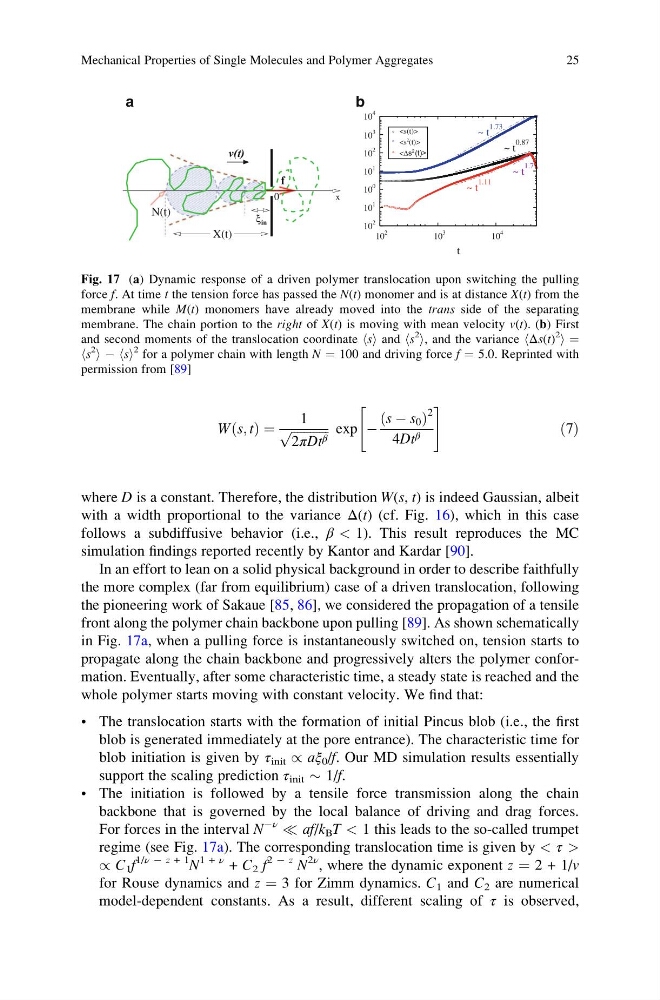
front along the polymer chain backbone upon pulling [89]. As shown schematically
in Fig. 17a, when a pulling force is instantaneously switched on, tension starts to
propagate along the chain backbone and progressively alters the polymer conformation. Eventually, after some characteristic time, a steady state is reached and the
whole polymer starts moving with constant velocity. We find that:
• The translocation starts with the formation of initial Pincus blob (i.e., the first
blob is generated immediately at the pore entrance). The characteristic time for
blob initiation is given by τ init / aξ 0 /f. Our MD simulation results essentially
support the scaling prediction τ init $ 1/f.
• The initiation is followed by a tensile force transmission along the chain
backbone that is governed by the local balance of driving and drag forces.
For forces in the interval N
Àν
( af/k B T < 1 this leads to the so-called trumpet
regime (see Fig. 17a). The corresponding translocation time is given by < τ >
/ C 1 f
1/ν À z + 1 N
1 + ν + C 2 f
2 À z N
2ν , where the dynamic exponent z ¼ 2 + 1/v
for Rouse dynamics and z ¼ 3 for Zimm dynamics. C 1 and C 2 are numerical
model-dependent constants. As a result, different scaling of τ is observed,
x
X(t)
N(t)
0
f
v(t)
ξ in
t
10
4
10
3
10
2
10
1
10
0
10
1
10
2
10
2
10
3
10
4
<Δs 2 (t)>
~ t
0.87
~ t
1.11
~ t
1.73
~ t
1.7
b
a
Fig. 17 (a) Dynamic response of a driven polymer translocation upon switching the pulling
force f. At time t the tension force has passed the N(t) monomer and is at distance X(t) from the
membrane while M(t) monomers have already moved into the trans side of the separating
membrane. The chain portion to the right of X(t) is moving with mean velocity v(t). (b) First
and second moments of the translocation coordinate hsi and hs
2
i, and the variance hΔs(t)
2
i ¼
hs
2 i À hsi
2 for a polymer chain with length N ¼ 100 and driving force f ¼ 5.0. Reprinted with
permission from [89]
Mechanical Properties of Single Molecules and Polymer Aggregates
25
ð Þ ¼
1
ffiffiffiffiffiffiffiffiffiffiffiffi
2πDt β
p
exp À
s À s 0
ð
Þ
2
4Dt β
"
#
ð7Þ
where D is a constant. Therefore, the distribution W(s, t) is indeed Gaussian, albeit
with a width proportional to the variance Δ(t) (cf. Fig. 16), which in this case
follows a subdiffusive behavior (i.e., β < 1). This result reproduces the MC
simulation findings reported recently by Kantor and Kardar [90].
In an effort to lean on a solid physical background in order to describe faithfully
the more complex (far from equilibrium) case of a driven translocation, following
the pioneering work of Sakaue [85, 86], we considered the propagation of a tensile
front along the polymer chain backbone upon pulling [89]. As shown schematically
in Fig. 17a, when a pulling force is instantaneously switched on, tension starts to
propagate along the chain backbone and progressively alters the polymer conformation. Eventually, after some characteristic time, a steady state is reached and the
whole polymer starts moving with constant velocity. We find that:
• The translocation starts with the formation of initial Pincus blob (i.e., the first
blob is generated immediately at the pore entrance). The characteristic time for
blob initiation is given by τ init / aξ 0 /f. Our MD simulation results essentially
support the scaling prediction τ init $ 1/f.
• The initiation is followed by a tensile force transmission along the chain
backbone that is governed by the local balance of driving and drag forces.
For forces in the interval N
Àν
( af/k B T < 1 this leads to the so-called trumpet
regime (see Fig. 17a). The corresponding translocation time is given by < τ >
/ C 1 f
1/ν À z + 1 N
1 + ν + C 2 f
2 À z N
2ν , where the dynamic exponent z ¼ 2 + 1/v
for Rouse dynamics and z ¼ 3 for Zimm dynamics. C 1 and C 2 are numerical
model-dependent constants. As a result, different scaling of τ is observed,
x
X(t)
N(t)
0
f
v(t)
ξ in
t
10
4
10
3
10
2
10
1
10
0
10
1
10
2
10
2
10
3
10
4
<Δs 2 (t)>
~ t
0.87
~ t
1.11
~ t
1.73
~ t
1.7
b
a
Fig. 17 (a) Dynamic response of a driven polymer translocation upon switching the pulling
force f. At time t the tension force has passed the N(t) monomer and is at distance X(t) from the
membrane while M(t) monomers have already moved into the trans side of the separating
membrane. The chain portion to the right of X(t) is moving with mean velocity v(t). (b) First
and second moments of the translocation coordinate hsi and hs
2
i, and the variance hΔs(t)
2
i ¼
hs
2 i À hsi
2 for a polymer chain with length N ¼ 100 and driving force f ¼ 5.0. Reprinted with
permission from [89]
Mechanical Properties of Single Molecules and Polymer Aggregates
25