

a nonlinear regime (first proposed by Pincus [24]) occurs, where X
h i=L / f ‘ p =k B T
À
Á 2=3
‘ p =R
∗
À
Á 1=3 with R
∗
/ ‘
2
p =D (in d ¼ 3). However, this Pincus regime is only
observable for n p > n p *. In d ¼ 2 dimensions, the nonlinear Pincus regime is
described simply by X
h i=L / f ‘ p =k B T
À
Á 1=3 , and this regime extends until saturation
of hXi at L starts. So, in d ¼ 2, the Kratky–Porod model also fails completely
with respect to the force–extension behavior, whereas in d ¼ 3 it holds for very stiff
and thin chains (for which n p * ) 1), if they are not too long (n p < n p *).
The various crossover predictions and the numerical evidence that we have
obtained for these crossovers are described in detail in two long papers [20, 22];
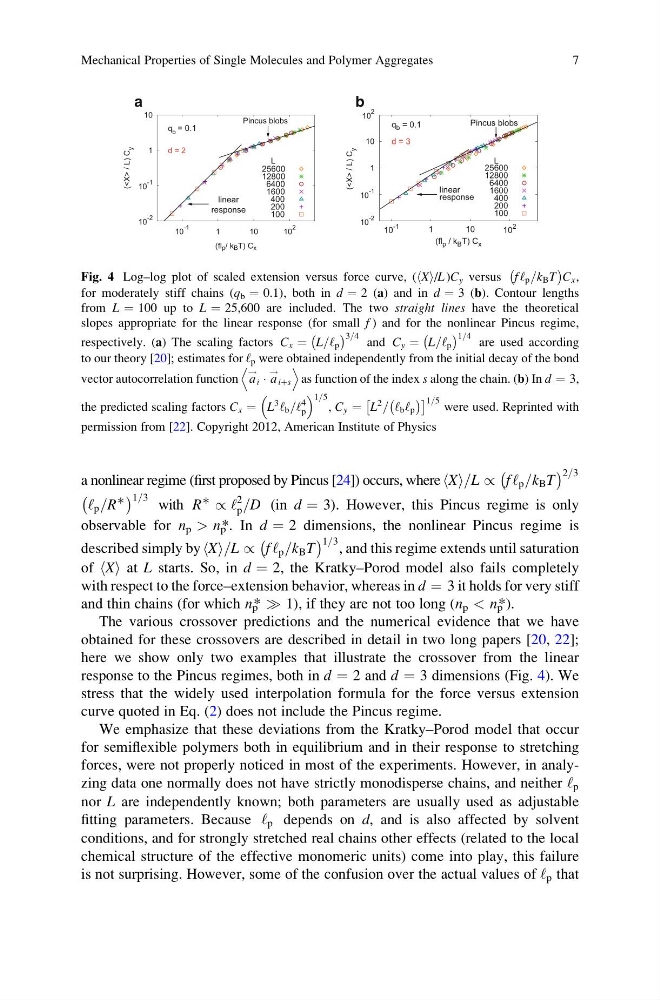
here we show only two examples that illustrate the crossover from the linear
response to the Pincus regimes, both in d ¼ 2 and d ¼ 3 dimensions (Fig. 4). We
stress that the widely used interpolation formula for the force versus extension
curve quoted in Eq. (2) does not include the Pincus regime.
We emphasize that these deviations from the Kratky–Porod model that occur
for semiflexible polymers both in equilibrium and in their response to stretching
forces, were not properly noticed in most of the experiments. However, in analyzing data one normally does not have strictly monodisperse chains, and neither ‘ p
nor L are independently known; both parameters are usually used as adjustable
fitting parameters. Because ‘ p depends on d, and is also affected by solvent
conditions, and for strongly stretched real chains other effects (related to the local
chemical structure of the effective monomeric units) come into play, this failure
is not surprising. However, some of the confusion over the actual values of ‘ p that
10
-2
10
-1
1
10
10
-2
10
-1
1
10
2
10
10
-1
1
10
2
10
( / L) C
y
( / L) C
y
(fl p / k B T) C x
linear
response
Pincus blobs
L
q b = 0.1
d = 2
25600
12800
6400
1600
400
200
100
10
-1
1
10
10
2
(fl p / k B T) C x
linear
response
Pincus blobs
L
q b = 0.1
d = 3
25600
12800
6400
1600
400
200
100
a
b
Fig. 4 Log–log plot of scaled extension versus force curve, (hXi/L )C y versus f ‘ p =k B T
À
Á
C x ,
for moderately stiff chains (q b ¼ 0.1), both in d ¼ 2 (a) and in d ¼ 3 (b). Contour lengths
from L ¼ 100 up to L ¼ 25,600 are included. The two straight lines have the theoretical
slopes appropriate for the linear response (for small f ) and for the nonlinear Pincus regime,
respectively. (a) The scaling factors C x ¼ L=‘ p
À
Á 3=4 and C y ¼ L=‘ p
À
Á 1=4 are used according
to our theory [20]; estimates for ‘ p were obtained independently from the initial decay of the bond
vector autocorrelation function a
!
i Á a
!
iþs
D
E
as function of the index s along the chain. (b) In d ¼ 3,
the predicted scaling factors C x ¼ L
3 ‘ b =‘
4
p
1=5
, C y ¼ L
2 = ‘ b ‘ p
À
Á
Â
à 1=5 were used. Reprinted with
permission from [22]. Copyright 2012, American Institute of Physics
Mechanical Properties of Single Molecules and Polymer Aggregates
7
h i=L / f ‘ p =k B T
À
Á 2=3
‘ p =R
∗
À
Á 1=3 with R
∗
/ ‘
2
p =D (in d ¼ 3). However, this Pincus regime is only
observable for n p > n p *. In d ¼ 2 dimensions, the nonlinear Pincus regime is
described simply by X
h i=L / f ‘ p =k B T
À
Á 1=3 , and this regime extends until saturation
of hXi at L starts. So, in d ¼ 2, the Kratky–Porod model also fails completely
with respect to the force–extension behavior, whereas in d ¼ 3 it holds for very stiff
and thin chains (for which n p * ) 1), if they are not too long (n p < n p *).
The various crossover predictions and the numerical evidence that we have
obtained for these crossovers are described in detail in two long papers [20, 22];
here we show only two examples that illustrate the crossover from the linear
response to the Pincus regimes, both in d ¼ 2 and d ¼ 3 dimensions (Fig. 4). We
stress that the widely used interpolation formula for the force versus extension
curve quoted in Eq. (2) does not include the Pincus regime.
We emphasize that these deviations from the Kratky–Porod model that occur
for semiflexible polymers both in equilibrium and in their response to stretching
forces, were not properly noticed in most of the experiments. However, in analyzing data one normally does not have strictly monodisperse chains, and neither ‘ p
nor L are independently known; both parameters are usually used as adjustable
fitting parameters. Because ‘ p depends on d, and is also affected by solvent
conditions, and for strongly stretched real chains other effects (related to the local
chemical structure of the effective monomeric units) come into play, this failure
is not surprising. However, some of the confusion over the actual values of ‘ p that
10
-2
10
-1
1
10
10
-2
10
-1
1
10
2
10
10
-1
1
10
2
10
(
y
(
y
(fl p / k B T) C x
linear
response
Pincus blobs
L
q b = 0.1
d = 2
25600
12800
6400
1600
400
200
100
10
-1
1
10
10
2
(fl p / k B T) C x
linear
response
Pincus blobs
L
q b = 0.1
d = 3
25600
12800
6400
1600
400
200
100
a
b
Fig. 4 Log–log plot of scaled extension versus force curve, (hXi/L )C y versus f ‘ p =k B T
À
Á
C x ,
for moderately stiff chains (q b ¼ 0.1), both in d ¼ 2 (a) and in d ¼ 3 (b). Contour lengths
from L ¼ 100 up to L ¼ 25,600 are included. The two straight lines have the theoretical
slopes appropriate for the linear response (for small f ) and for the nonlinear Pincus regime,
respectively. (a) The scaling factors C x ¼ L=‘ p
À
Á 3=4 and C y ¼ L=‘ p
À
Á 1=4 are used according
to our theory [20]; estimates for ‘ p were obtained independently from the initial decay of the bond
vector autocorrelation function a
!
i Á a
!
iþs
D
E
as function of the index s along the chain. (b) In d ¼ 3,
the predicted scaling factors C x ¼ L
3 ‘ b =‘
4
p
1=5
, C y ¼ L
2 = ‘ b ‘ p
À
Á
Â
à 1=5 were used. Reprinted with
permission from [22]. Copyright 2012, American Institute of Physics
Mechanical Properties of Single Molecules and Polymer Aggregates
7