

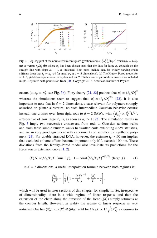
occurs (at n p ¼ n p
* , see Fig. 3b). Flory theory [21, 22] predicts that n
Ã
p / ‘ p =D
À
Á 2
whereas the simulations seem to suggest that n
Ã
p / ‘ p =D
À
Á 2:5 [22]. It is also
important to note that in d ¼ 2 dimensions, a case relevant for polymers strongly
adsorbed on planar substrates, no such intermediate Gaussian behavior occurs;
instead, one crosses over from rigid rods to d ¼ 2 SAWs, with R
2
g
D E
/ ‘
1=2
p L
3=2 ,
irrespective of how large ‘ p is, as soon as n p > 1 [22]. The simulation results in
Fig. 3 imply two successive crossovers, from rods to Gaussian random walks
and from these simple random walks to swollen coils exhibiting SAW statistics,
and are in very good agreement with experiments on semiflexible synthetic polymers [23]. For double-stranded DNA, however, the estimate l p % 50 nm implies
that excluded volume effects become important only if L exceeds 100 nm. These
deviations from the Kratky–Porod model also invalidate its predictions for the
force versus extension curve [1, 2]:
X
h i=L / f ‘ p =k B T small f
ð
Þ , 1 À const f ‘ p =k B T
À
Á À 1=2
ð
Þ large f
ð
Þ :
ð1Þ
In d ¼ 3 dimensions, a useful interpolation formula between both regimes is:
f ‘ p
k B T
¼
1
4
1 À
X
h i
L
À2
þ
X
h i
L
À
1
4
"
#
,
ð2Þ
which will be used in later sections of this chapter for simplicity. So, irrespective
of dimensionality, there is a wide regime of linear response and then the
extension of the chain along the direction of the force (hXi) simply saturates at
the contour length. However, in reality the regime of linear response is very
restricted: One has hXi/L / (hR e
2 i/L)f/k B T until for f =k B T / 1=
ffiffiffiffiffiffiffiffiffi ffi
R
2
e
q
a crossover to
0.4
0.2
0.1
0.05
0.03
0.02
0.01
0.005
10 -3
10 -2
10 -1
1
10
10 -1
10 -2
10 -2
1
10 4
10 10 2 10 3
3< R
g
2
> / (lp L)
3< R
g
2
> / (lp L)
np
q b
q b
slope = 2ν-1
WLC
0.75
1
2
3
5
1
10 2
10 4
n p / n* p
slope = 2ν-1
0.2
0.1
0.05
0.03
0.02
0.01
0.005
b
a
Fig. 3 Log–log plot of the normalized mean square gyration radius 3 R
2
g
D E
= ‘ p L
À Á
versus n p ¼ L=‘ p
(a) or versus n p /n
Ã
p (b) where n
Ã
p has been chosen such that the data for large n p coincide on the
straight line with slope 2v À 1, as indicated. Both parts include data for widely varying chain
stiffness (note that ‘ p % q
À1
b =4 for small q b in d ¼ 3 dimensions). (a) The Kratky–Porod model for
all L, ‘ p yields a unique master curve, denoted WLC. The horizontal part of this curve is also included
in (b). Reprinted with permission from [20]. Copyright 2012, American Institute of Physics
6
R. Berger et al.
* , see Fig. 3b). Flory theory [21, 22] predicts that n
Ã
p / ‘ p =D
À
Á 2
whereas the simulations seem to suggest that n
Ã
p / ‘ p =D
À
Á 2:5 [22]. It is also
important to note that in d ¼ 2 dimensions, a case relevant for polymers strongly
adsorbed on planar substrates, no such intermediate Gaussian behavior occurs;
instead, one crosses over from rigid rods to d ¼ 2 SAWs, with R
2
g
D E
/ ‘
1=2
p L
3=2 ,
irrespective of how large ‘ p is, as soon as n p > 1 [22]. The simulation results in
Fig. 3 imply two successive crossovers, from rods to Gaussian random walks
and from these simple random walks to swollen coils exhibiting SAW statistics,
and are in very good agreement with experiments on semiflexible synthetic polymers [23]. For double-stranded DNA, however, the estimate l p % 50 nm implies
that excluded volume effects become important only if L exceeds 100 nm. These
deviations from the Kratky–Porod model also invalidate its predictions for the
force versus extension curve [1, 2]:
X
h i=L / f ‘ p =k B T small f
ð
Þ , 1 À const f ‘ p =k B T
À
Á À 1=2
ð
Þ large f
ð
Þ :
ð1Þ
In d ¼ 3 dimensions, a useful interpolation formula between both regimes is:
f ‘ p
k B T
¼
1
4
1 À
X
h i
L
À2
þ
X
h i
L
À
1
4
"
#
,
ð2Þ
which will be used in later sections of this chapter for simplicity. So, irrespective
of dimensionality, there is a wide regime of linear response and then the
extension of the chain along the direction of the force (hXi) simply saturates at
the contour length. However, in reality the regime of linear response is very
restricted: One has hXi/L / (hR e
2 i/L)f/k B T until for f =k B T / 1=
ffiffiffiffiffiffiffiffiffi ffi
R
2
e
q
a crossover to
0.4
0.2
0.1
0.05
0.03
0.02
0.01
0.005
10 -3
10 -2
10 -1
1
10
10 -1
10 -2
10 -2
1
10 4
10 10 2 10 3
3< R
g
2
> / (lp L)
3< R
g
2
> / (lp L)
np
q b
q b
slope = 2ν-1
WLC
0.75
1
2
3
5
1
10 2
10 4
n p / n* p
slope = 2ν-1
0.2
0.1
0.05
0.03
0.02
0.01
0.005
b
a
Fig. 3 Log–log plot of the normalized mean square gyration radius 3 R
2
g
D E
= ‘ p L
À Á
versus n p ¼ L=‘ p
(a) or versus n p /n
Ã
p (b) where n
Ã
p has been chosen such that the data for large n p coincide on the
straight line with slope 2v À 1, as indicated. Both parts include data for widely varying chain
stiffness (note that ‘ p % q
À1
b =4 for small q b in d ¼ 3 dimensions). (a) The Kratky–Porod model for
all L, ‘ p yields a unique master curve, denoted WLC. The horizontal part of this curve is also included
in (b). Reprinted with permission from [20]. Copyright 2012, American Institute of Physics
6
R. Berger et al.