

be the “gold standard” for stiff polymers [68], is rather restricted. So it turns out that
the exponential decay of the bond autocorrelation function hcos(θ(s))i for bonds
along the backbone s steps of length l b apart, hcos(θ(s))i ~ exp(Às l b /l p ), is delicate.
Such an exponential decay can only be found for a rather small number of steps
[66], s < l p /l b , but is not asymptotically for s ! 1, where the decay always
follows a power law hcos(θ(s)i / s
À β with β ¼ 2 À 2ν % 0.824 under good
solvent conditions but β ¼ 3/2 for theta solvents [66]. A Gaussian behavior
(as predicted by the Kratky–Porod model) occurs only for polymers in 3D space
that are both very stiff and very thin, namely for the contour lengths L in the range
l p ( L ( (l p /R cs )
2 l p [70]. Only in this regime (and in the rather trivial regime
L < l p , where the polymer resembles a rigid rod of length l p ) would the
Kratky–Porod model be applicable. As we shall see below, for bottlebrush
polymers the persistence length (l p ) is not very much larger than their crosssectional radius (R cs ), and then the Kratky–Porod model fails.
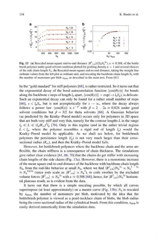
However, for bottlebrush polymers where the backbone chain and the arms are
flexible, the chain stiffness is a consequence of chain thickness. The simulations
give rather clear evidence [61, 66, 70] that the chains do get stiffer with increasing
chain lengths of the side chains (Fig. 13a). However, there is a monotonic increase
of the mean square end-to-end distance of the backbone with backbone chain length
N b , from the rod-like behavior at small N b , where we find hR
2
e,b i/N b
2ν
/ N b
2 À 2ν
% N b
0.824 (since rods scale as hR
2
e,b i / N b
2 ), to coils swollen by the excluded
volume forces hR
2
e,b i / N b
2ν with ν % 0.588 [68]; hence, for hR
2
e,b i/N b
2ν horizontal plateaus result, as is evident from the data.
It turns out that there is a simple rescaling possible, by which all curves
superimpose (at least approximately) on a master curve (Fig. 13b): N b is rescaled
by s blob , the number of monomers per blob, motivated by the idea that the
bottlebrush polymer is viewed as a pearl-necklace chain of blobs, the blob radius
being the cross-sectional radius of the cylindrical brush. From this condition, s blob is
easily derived numerically from the simulation data.
Fig. 13 (a) Rescaled mean-square end-to-end distance hR
2
e,b i/(2l b N b
2ν ), ν % 0.588, of the bottle
brush polymer under good solvent condition plotted for grafting density σ ¼ 1 and several choices
of the side chain length N s . (b) Rescaled mean-square end-to-end distance, taking the straight line
ordinate values from the left plot as ordinate unit, and rescaling the backbone chain length N b with
the number of monomers per blob s blob , as described in the main text. From [61]
134
K. Binder et al.
the exponential decay of the bond autocorrelation function hcos(θ(s))i for bonds
along the backbone s steps of length l b apart, hcos(θ(s))i ~ exp(Às l b /l p ), is delicate.
Such an exponential decay can only be found for a rather small number of steps
[66], s < l p /l b , but is not asymptotically for s ! 1, where the decay always
follows a power law hcos(θ(s)i / s
À β with β ¼ 2 À 2ν % 0.824 under good
solvent conditions but β ¼ 3/2 for theta solvents [66]. A Gaussian behavior
(as predicted by the Kratky–Porod model) occurs only for polymers in 3D space
that are both very stiff and very thin, namely for the contour lengths L in the range
l p ( L ( (l p /R cs )
2 l p [70]. Only in this regime (and in the rather trivial regime
L < l p , where the polymer resembles a rigid rod of length l p ) would the
Kratky–Porod model be applicable. As we shall see below, for bottlebrush
polymers the persistence length (l p ) is not very much larger than their crosssectional radius (R cs ), and then the Kratky–Porod model fails.
However, for bottlebrush polymers where the backbone chain and the arms are
flexible, the chain stiffness is a consequence of chain thickness. The simulations
give rather clear evidence [61, 66, 70] that the chains do get stiffer with increasing
chain lengths of the side chains (Fig. 13a). However, there is a monotonic increase
of the mean square end-to-end distance of the backbone with backbone chain length
N b , from the rod-like behavior at small N b , where we find hR
2
e,b i/N b
2ν
/ N b
2 À 2ν
% N b
0.824 (since rods scale as hR
2
e,b i / N b
2 ), to coils swollen by the excluded
volume forces hR
2
e,b i / N b
2ν with ν % 0.588 [68]; hence, for hR
2
e,b i/N b
2ν horizontal plateaus result, as is evident from the data.
It turns out that there is a simple rescaling possible, by which all curves
superimpose (at least approximately) on a master curve (Fig. 13b): N b is rescaled
by s blob , the number of monomers per blob, motivated by the idea that the
bottlebrush polymer is viewed as a pearl-necklace chain of blobs, the blob radius
being the cross-sectional radius of the cylindrical brush. From this condition, s blob is
easily derived numerically from the simulation data.
Fig. 13 (a) Rescaled mean-square end-to-end distance hR
2
e,b i/(2l b N b
2ν ), ν % 0.588, of the bottle
brush polymer under good solvent condition plotted for grafting density σ ¼ 1 and several choices
of the side chain length N s . (b) Rescaled mean-square end-to-end distance, taking the straight line
ordinate values from the left plot as ordinate unit, and rescaling the backbone chain length N b with
the number of monomers per blob s blob , as described in the main text. From [61]
134
K. Binder et al.