4.3 Popular Kernels
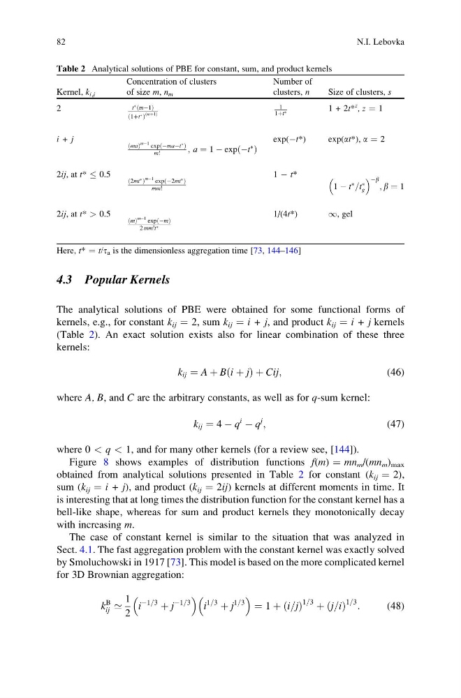
The analytical solutions of PBE were obtained for some functional forms of
kernels, e.g., for constant k ij ¼ 2, sum k ij ¼ i + j, and product k ij ¼ i + j kernels
(Table 2). An exact solution exists also for linear combination of these three
kernels:
k ij ¼ A þ Bði þ jÞ þ Cij;
(46)
where A, B, and C are the arbitrary constants, as well as for q-sum kernel:
k ij ¼ 4 À q
i
À q
j
;
(47)
where 0 < q < 1, and for many other kernels (for a review see, [144]).
Figure 8 shows examples of distribution functions f(m) ¼ mn m /(mn m ) max
obtained from analytical solutions presented in Table 2 for constant (k ij ¼ 2),
sum (k ij ¼ i + j), and product (k ij ¼ 2ij) kernels at different moments in time. It
is interesting that at long times the distribution function for the constant kernel has a
bell-like shape, whereas for sum and product kernels they monotonically decay
with increasing m.
The case of constant kernel is similar to the situation that was analyzed in
Sect. 4.1. The fast aggregation problem with the constant kernel was exactly solved
by Smoluchowski in 1917 [73]. This model is based on the more complicated kernel
for 3D Brownian aggregation:
k
B
ij ’
1
2
i
À1=3
þ j
À1=3
i
1=3
þ j
1=3
¼ 1 þ i=j
ð Þ
1=3 þ j=i
ð Þ
1=3 :
(48)
Table 2 Analytical solutions of PBE for constant, sum, and product kernels
Kernel, k i,j
Concentration of clusters
of size m, n m
Number of
clusters, n
Size of clusters, s
2
t
à ðmÀ1Þ
1þt Ã
ð
Þ
mþ1
ð
Þ
1
1þt Ã
1 + 2t*
z , z ¼ 1
i + j
ma
ð Þ
mÀ1 exp ÀmaÀt
Ã
ð
Þ
m!
; a ¼ 1 À exp Àt
Ã
ð Þ
exp(Àt*)
exp(at*), a ¼ 2
2ij, at t* 0.5
2mt
Ã
ð
Þ
mÀ1 exp À2mt
Ã
ð
Þ
mm!
1 À t*
1 À t
à =t
Ã
g
Àb ; b ¼ 1
2ij, at t* > 0.5
ðmÞ
mÀ1 exp Àm
ð Þ
2 mm!t Ã
1/(4t*)
1, gel
Here, t* ¼ t/t a is the dimensionless aggregation time [73, 144–146]
82
N.I. Lebovka