

The prime at the second sum indicates that the terms with m ¼ 0 have to be
multiplied by 1/2 and the term with m ¼ l ¼ 0 is not counted in the sum because
it is included in the uniform part of the potential [59]. In the sum over m, only terms
with m ¼ jN s contribute, where j is an integer. J lm is given by:
J lm ¼
ð 1
À1
P
m
l ðxÞ dx;
(91)
which can be expressed in terms of gamma functions and generalized hypergeometric
functions [59, 153].
With (56), we obtain the electrostatic energy:
E el ¼ E 0 ð1 À ^ yÞ
2
À
16p
3 a
2 s
2
s
^
y
2
E
X 1
l¼0
X l
m¼0
0 d m; jN s
k l
J
2
lm
ð2l þ 1Þ
4p
ðl À mÞ!
ðl þ mÞ!
K lþ1=2 ðkaÞ
ffiffiffiffiffi ffi
ka
p
:
(92)
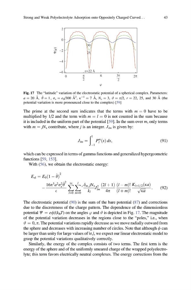
The electrostatic potential (90) is the sum of the bare potential (87) and corrections
due to the discreteness of the charge pattern. The dependence of the dimensionless
potential C ¼ ef/(k B T) on the angles ’ and # is depicted in Fig. 17. The magnitude
of the potential variation decreases in the regions close to the “poles,” i.e., when
# ¼ 0, p. The potential variations rapidly decrease as we move radially outward from
the sphere and decreases with increasing number of circles. Note that although f can
be larger than unity for large values of |s s |, we expect our linear electrostatic model to
grasp the potential variations qualitatively correctly.
Similarly, the energy of the complex consists of two terms. The first term is the
energy of the sphere and of the uniformly smeared charge of the wrapped polyelectrolyte; this term favors electrically neutral complexes. The energy corrections from the
r 22
25
30
0
2
3
2
2
6
4
2
0
2
p
p
p
p
Fig. 17 The “latitude” variation of the electrostatic potential of a spherical complex. Parameters:
a ¼ 20 A ˚ , ^
y ¼ 1 , s s ¼ e 0 /300 A ˚ 2 , k
À1 ¼ 7 A ˚ , N c ¼ 3, # ¼ p/2, r ¼ 22, 25, and 30 A ˚ (the
potential variation is more pronounced close to the complex) [59]
Strong and Weak Polyelectrolyte Adsorption onto Oppositely Charged Curved. . .
43
multiplied by 1/2 and the term with m ¼ l ¼ 0 is not counted in the sum because
it is included in the uniform part of the potential [59]. In the sum over m, only terms
with m ¼ jN s contribute, where j is an integer. J lm is given by:
J lm ¼
ð 1
À1
P
m
l ðxÞ dx;
(91)
which can be expressed in terms of gamma functions and generalized hypergeometric
functions [59, 153].
With (56), we obtain the electrostatic energy:
E el ¼ E 0 ð1 À ^ yÞ
2
À
16p
3 a
2 s
2
s
^
y
2
E
X 1
l¼0
X l
m¼0
0 d m; jN s
k l
J
2
lm
ð2l þ 1Þ
4p
ðl À mÞ!
ðl þ mÞ!
K lþ1=2 ðkaÞ
ffiffiffiffiffi ffi
ka
p
:
(92)
The electrostatic potential (90) is the sum of the bare potential (87) and corrections
due to the discreteness of the charge pattern. The dependence of the dimensionless
potential C ¼ ef/(k B T) on the angles ’ and # is depicted in Fig. 17. The magnitude
of the potential variation decreases in the regions close to the “poles,” i.e., when
# ¼ 0, p. The potential variations rapidly decrease as we move radially outward from
the sphere and decreases with increasing number of circles. Note that although f can
be larger than unity for large values of |s s |, we expect our linear electrostatic model to
grasp the potential variations qualitatively correctly.
Similarly, the energy of the complex consists of two terms. The first term is the
energy of the sphere and of the uniformly smeared charge of the wrapped polyelectrolyte; this term favors electrically neutral complexes. The energy corrections from the
r 22
25
30
0
2
3
2
2
6
4
2
0
2
p
p
p
p
Fig. 17 The “latitude” variation of the electrostatic potential of a spherical complex. Parameters:
a ¼ 20 A ˚ , ^
y ¼ 1 , s s ¼ e 0 /300 A ˚ 2 , k
À1 ¼ 7 A ˚ , N c ¼ 3, # ¼ p/2, r ¼ 22, 25, and 30 A ˚ (the
potential variation is more pronounced close to the complex) [59]
Strong and Weak Polyelectrolyte Adsorption onto Oppositely Charged Curved. . .
43