

considered, but evaluation of the resulting energy expressions may be rather
cumbersome.
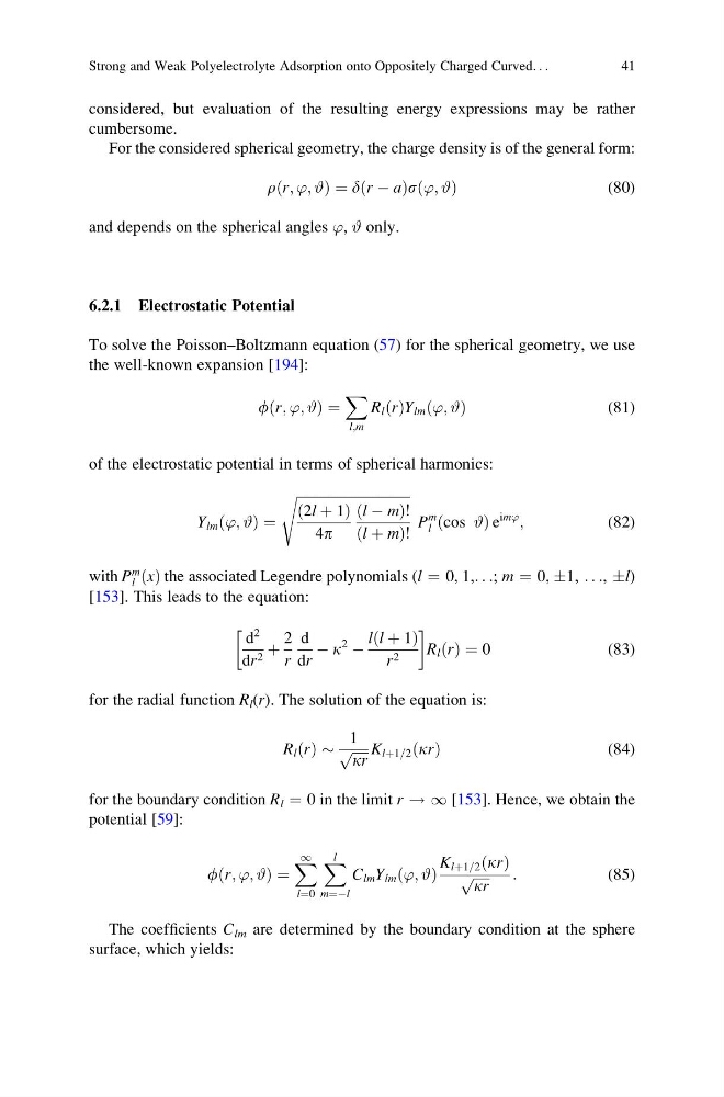
For the considered spherical geometry, the charge density is of the general form:
rðr; ’; #Þ ¼ dðr À aÞsð’; #Þ
(80)
and depends on the spherical angles ’, # only.
6.2.1 Electrostatic Potential
To solve the Poisson–Boltzmann equation (57) for the spherical geometry, we use
the well-known expansion [194]:
fðr; ’; #Þ ¼
X
l;m
R l ðrÞY lm ð’; #Þ
(81)
of the electrostatic potential in terms of spherical harmonics:
Y lm ð’; #Þ ¼
ffiffiffiffiffiffiffiffiffiffiffiffiffiffiffiffiffiffiffiffiffiffiffiffiffiffiffiffiffiffiffiffiffi
ð2l þ 1Þ
4p
ðl À mÞ!
ðl þ mÞ!
s
P
m
l ðcos #Þ e
im’
;
(82)
with P
m
l ðxÞ the associated Legendre polynomials (l ¼ 0, 1,. . .; m ¼ 0, Æ1, . . ., Æl)
[153]. This leads to the equation:
d
2
dr 2 þ
2
r
d
dr
À k
2
À
lðl þ 1Þ
r 2
!
R l ðrÞ ¼ 0
(83)
for the radial function R l (r). The solution of the equation is:
R l ðrÞ $
1
ffiffiffiffiffi
kr
p K lþ1=2 ðkrÞ
(84)
for the boundary condition R l ¼ 0 in the limit r ! 1 [153]. Hence, we obtain the
potential [59]:
fðr; ’; #Þ ¼
X 1
l¼0
X l
m¼Àl
C lm Y lm ð’; #Þ
K lþ1=2 ðkrÞ
ffiffiffiffiffi
kr
p
:
(85)
The coefficients C lm are determined by the boundary condition at the sphere
surface, which yields:
Strong and Weak Polyelectrolyte Adsorption onto Oppositely Charged Curved. . .
41
cumbersome.
For the considered spherical geometry, the charge density is of the general form:
rðr; ’; #Þ ¼ dðr À aÞsð’; #Þ
(80)
and depends on the spherical angles ’, # only.
6.2.1 Electrostatic Potential
To solve the Poisson–Boltzmann equation (57) for the spherical geometry, we use
the well-known expansion [194]:
fðr; ’; #Þ ¼
X
l;m
R l ðrÞY lm ð’; #Þ
(81)
of the electrostatic potential in terms of spherical harmonics:
Y lm ð’; #Þ ¼
ffiffiffiffiffiffiffiffiffiffiffiffiffiffiffiffiffiffiffiffiffiffiffiffiffiffiffiffiffiffiffiffiffi
ð2l þ 1Þ
4p
ðl À mÞ!
ðl þ mÞ!
s
P
m
l ðcos #Þ e
im’
;
(82)
with P
m
l ðxÞ the associated Legendre polynomials (l ¼ 0, 1,. . .; m ¼ 0, Æ1, . . ., Æl)
[153]. This leads to the equation:
d
2
dr 2 þ
2
r
d
dr
À k
2
À
lðl þ 1Þ
r 2
!
R l ðrÞ ¼ 0
(83)
for the radial function R l (r). The solution of the equation is:
R l ðrÞ $
1
ffiffiffiffiffi
kr
p K lþ1=2 ðkrÞ
(84)
for the boundary condition R l ¼ 0 in the limit r ! 1 [153]. Hence, we obtain the
potential [59]:
fðr; ’; #Þ ¼
X 1
l¼0
X l
m¼Àl
C lm Y lm ð’; #Þ
K lþ1=2 ðkrÞ
ffiffiffiffiffi
kr
p
:
(85)
The coefficients C lm are determined by the boundary condition at the sphere
surface, which yields:
Strong and Weak Polyelectrolyte Adsorption onto Oppositely Charged Curved. . .
41