

4.4 Spherical Surface
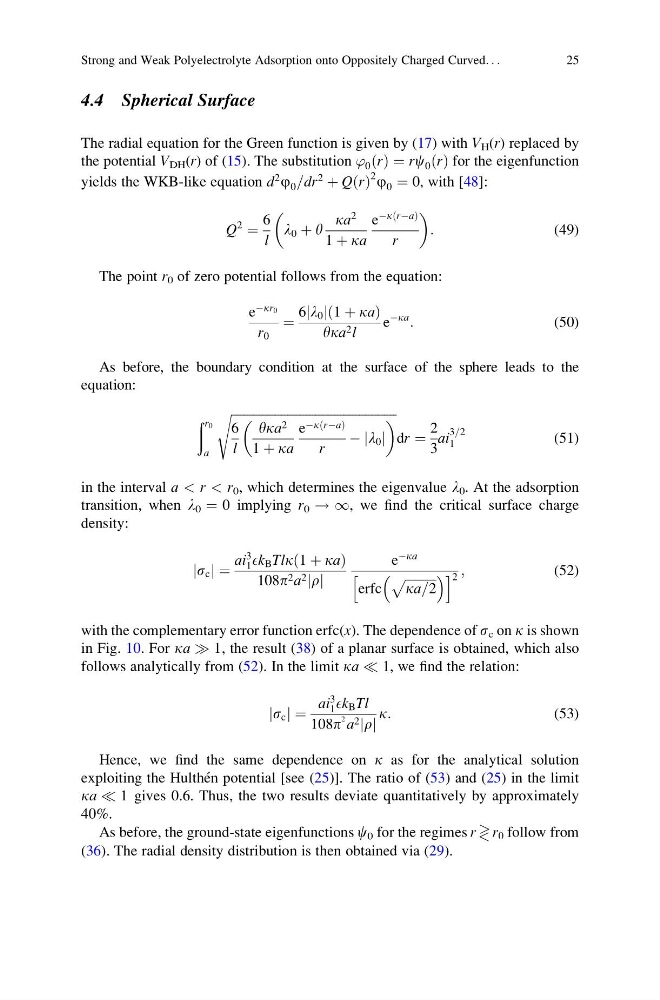
The radial equation for the Green function is given by (17) with V H (r) replaced by
the potential V DH (r) of (15). The substitution ’ 0 ðrÞ ¼ rc 0 ðrÞ for the eigenfunction
yields the WKB-like equation d
2
j 0 =dr
2
þ QðrÞ
2 j 0 ¼ 0, with [48]:
Q
2
¼
6
l
l 0 þ y
ka
2
1 þ ka
e
ÀkðrÀaÞ
r
:
(49)
The point r 0 of zero potential follows from the equation:
e
Àkr 0
r 0
¼
6jl 0 jð1 þ kaÞ
yka 2 l
e
Àka
:
(50)
As before, the boundary condition at the surface of the sphere leads to the
equation:
ð r 0
a
ffiffiffiffiffiffiffiffiffiffiffiffiffiffiffiffiffiffiffiffiffiffiffiffiffiffiffiffiffiffiffiffiffiffiffiffiffiffiffiffiffiffiffiffiffiffiffiffiffiffiffiffiffi
6
l
yka 2
1 þ ka
e ÀkðrÀaÞ
r
À jl 0 j
s
dr ¼
2
3
ai
3=2
1
(51)
in the interval a < r < r 0 , which determines the eigenvalue l 0 . At the adsorption
transition, when l 0 ¼ 0 implying r 0 ! 1, we find the critical surface charge
density:
js c j ¼
ai
3
1 Ek B Tlkð1 þ kaÞ
108p 2 a 2 jrj
e
Àka
erfc
ffiffiffiffiffiffiffiffiffiffi
ka=2
p
h
i 2 ;
(52)
with the complementary error function erfc(x). The dependence of s c on k is shown
in Fig. 10. For ka ) 1, the result (38) of a planar surface is obtained, which also
follows analytically from (52). In the limit ka ( 1, we find the relation:
js c j ¼
ai
3
1 Ek B Tl
108p
2 a 2 jrj
k:
(53)
Hence, we find the same dependence on k as for the analytical solution
exploiting the Hulthe ´n potential [see (25)]. The ratio of (53) and (25) in the limit
ka ( 1 gives 0.6. Thus, the two results deviate quantitatively by approximately
40%.
As before, the ground-state eigenfunctions c 0 for the regimes r >
< r 0 follow from
(36). The radial density distribution is then obtained via (29).
Strong and Weak Polyelectrolyte Adsorption onto Oppositely Charged Curved. . .
25
The radial equation for the Green function is given by (17) with V H (r) replaced by
the potential V DH (r) of (15). The substitution ’ 0 ðrÞ ¼ rc 0 ðrÞ for the eigenfunction
yields the WKB-like equation d
2
j 0 =dr
2
þ QðrÞ
2 j 0 ¼ 0, with [48]:
Q
2
¼
6
l
l 0 þ y
ka
2
1 þ ka
e
ÀkðrÀaÞ
r
:
(49)
The point r 0 of zero potential follows from the equation:
e
Àkr 0
r 0
¼
6jl 0 jð1 þ kaÞ
yka 2 l
e
Àka
:
(50)
As before, the boundary condition at the surface of the sphere leads to the
equation:
ð r 0
a
ffiffiffiffiffiffiffiffiffiffiffiffiffiffiffiffiffiffiffiffiffiffiffiffiffiffiffiffiffiffiffiffiffiffiffiffiffiffiffiffiffiffiffiffiffiffiffiffiffiffiffiffiffi
6
l
yka 2
1 þ ka
e ÀkðrÀaÞ
r
À jl 0 j
s
dr ¼
2
3
ai
3=2
1
(51)
in the interval a < r < r 0 , which determines the eigenvalue l 0 . At the adsorption
transition, when l 0 ¼ 0 implying r 0 ! 1, we find the critical surface charge
density:
js c j ¼
ai
3
1 Ek B Tlkð1 þ kaÞ
108p 2 a 2 jrj
e
Àka
erfc
ffiffiffiffiffiffiffiffiffiffi
ka=2
p
h
i 2 ;
(52)
with the complementary error function erfc(x). The dependence of s c on k is shown
in Fig. 10. For ka ) 1, the result (38) of a planar surface is obtained, which also
follows analytically from (52). In the limit ka ( 1, we find the relation:
js c j ¼
ai
3
1 Ek B Tl
108p
2 a 2 jrj
k:
(53)
Hence, we find the same dependence on k as for the analytical solution
exploiting the Hulthe ´n potential [see (25)]. The ratio of (53) and (25) in the limit
ka ( 1 gives 0.6. Thus, the two results deviate quantitatively by approximately
40%.
As before, the ground-state eigenfunctions c 0 for the regimes r >
< r 0 follow from
(36). The radial density distribution is then obtained via (29).
Strong and Weak Polyelectrolyte Adsorption onto Oppositely Charged Curved. . .
25