

4 Experimental Material Functions in Rubber Science
4.1 Material Functions in the Linear Viscoelastic Range
4.1.1 Shear Viscosity
In principle, the shear viscosity function in the linear viscoelastic range reduces to
the so-called pseudo-Newtonian shear viscosity, defined as: η 0 ¼ lim
_
γ!0
η _
γ
ð Þ. This
quantity is not a function per se but a material property that is directly related to
macromolecular characteristics, for instance the molecular weight and its distribution. The only relevant shear viscosity function in the linear domain is thus the
temperature dependent η 0 (T), for which the so-called Arrhenius approach is found
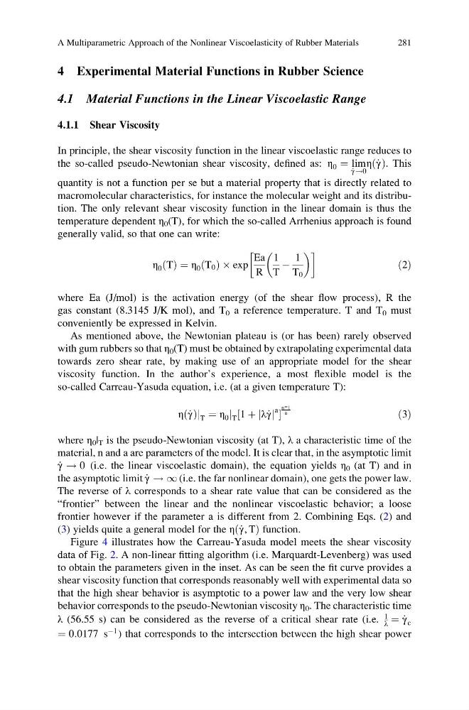
generally valid, so that one can write:
η 0 T
ð Þ ¼ η 0 T 0
ð Þ Â exp
Ea
R
1
T
À
1
T 0
ð2Þ
where Ea (J/mol) is the activation energy (of the shear flow process), R the
gas constant (8.3145 J/K mol), and T 0 a reference temperature. T and T 0 must
conveniently be expressed in Kelvin.
As mentioned above, the Newtonian plateau is (or has been) rarely observed
with gum rubbers so that η 0 (T) must be obtained by extrapolating experimental data
towards zero shear rate, by making use of an appropriate model for the shear
viscosity function. In the author’s experience, a most flexible model is the
so-called Carreau-Yasuda equation, i.e. (at a given temperature T):
η _
γ
ð Þj T ¼ η 0 j T 1 þ λ _
γ
j j
a
½
n-1
a
ð3Þ
where η 0 | T is the pseudo-Newtonian viscosity (at T), λ a characteristic time of the
material, n and a are parameters of the model. It is clear that, in the asymptotic limit
_
γ ! 0 (i.e. the linear viscoelastic domain), the equation yields η 0 (at T) and in
the asymptotic limit _
γ ! 1 (i.e. the far nonlinear domain), one gets the power law.
The reverse of λ corresponds to a shear rate value that can be considered as the
“frontier” between the linear and the nonlinear viscoelastic behavior; a loose
frontier however if the parameter a is different from 2. Combining Eqs. (2) and
(3) yields quite a general model for the ηð _
γ, TÞ function.
Figure 4 illustrates how the Carreau-Yasuda model meets the shear viscosity
data of Fig. 2. A non-linear fitting algorithm (i.e. Marquardt-Levenberg) was used
to obtain the parameters given in the inset. As can be seen the fit curve provides a
shear viscosity function that corresponds reasonably well with experimental data so
that the high shear behavior is asymptotic to a power law and the very low shear
behavior corresponds to the pseudo-Newtonian viscosity η 0 . The characteristic time
λ (56.55 s) can be considered as the reverse of a critical shear rate (i.e.
1
λ ¼ _
γ c
¼ 0:0177 s
À1 ) that corresponds to the intersection between the high shear power
A Multiparametric Approach of the Nonlinear Viscoelasticity of Rubber Materials
281
4.1 Material Functions in the Linear Viscoelastic Range
4.1.1 Shear Viscosity
In principle, the shear viscosity function in the linear viscoelastic range reduces to
the so-called pseudo-Newtonian shear viscosity, defined as: η 0 ¼ lim
_
γ!0
η _
γ
ð Þ. This
quantity is not a function per se but a material property that is directly related to
macromolecular characteristics, for instance the molecular weight and its distribution. The only relevant shear viscosity function in the linear domain is thus the
temperature dependent η 0 (T), for which the so-called Arrhenius approach is found
generally valid, so that one can write:
η 0 T
ð Þ ¼ η 0 T 0
ð Þ Â exp
Ea
R
1
T
À
1
T 0
ð2Þ
where Ea (J/mol) is the activation energy (of the shear flow process), R the
gas constant (8.3145 J/K mol), and T 0 a reference temperature. T and T 0 must
conveniently be expressed in Kelvin.
As mentioned above, the Newtonian plateau is (or has been) rarely observed
with gum rubbers so that η 0 (T) must be obtained by extrapolating experimental data
towards zero shear rate, by making use of an appropriate model for the shear
viscosity function. In the author’s experience, a most flexible model is the
so-called Carreau-Yasuda equation, i.e. (at a given temperature T):
η _
γ
ð Þj T ¼ η 0 j T 1 þ λ _
γ
j j
a
½
n-1
a
ð3Þ
where η 0 | T is the pseudo-Newtonian viscosity (at T), λ a characteristic time of the
material, n and a are parameters of the model. It is clear that, in the asymptotic limit
_
γ ! 0 (i.e. the linear viscoelastic domain), the equation yields η 0 (at T) and in
the asymptotic limit _
γ ! 1 (i.e. the far nonlinear domain), one gets the power law.
The reverse of λ corresponds to a shear rate value that can be considered as the
“frontier” between the linear and the nonlinear viscoelastic behavior; a loose
frontier however if the parameter a is different from 2. Combining Eqs. (2) and
(3) yields quite a general model for the ηð _
γ, TÞ function.
Figure 4 illustrates how the Carreau-Yasuda model meets the shear viscosity
data of Fig. 2. A non-linear fitting algorithm (i.e. Marquardt-Levenberg) was used
to obtain the parameters given in the inset. As can be seen the fit curve provides a
shear viscosity function that corresponds reasonably well with experimental data so
that the high shear behavior is asymptotic to a power law and the very low shear
behavior corresponds to the pseudo-Newtonian viscosity η 0 . The characteristic time
λ (56.55 s) can be considered as the reverse of a critical shear rate (i.e.
1
λ ¼ _
γ c
¼ 0:0177 s
À1 ) that corresponds to the intersection between the high shear power
A Multiparametric Approach of the Nonlinear Viscoelasticity of Rubber Materials
281