

4.8 The Wess-Zumino Model and a Problem of the Chiral Effective Potential
93
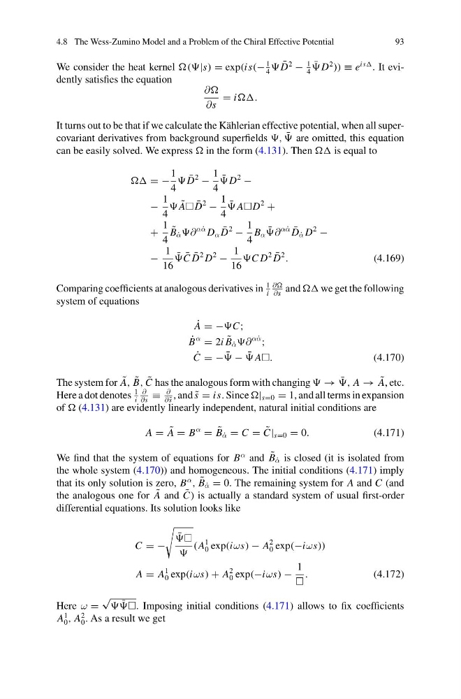
We consider the heat kernel = exp(is(−
1
4
¯
D
2
−
1
4
¯
D
2
)) ≡ e
is . It evidently satisfies the equation
∂
∂s
= i.
It turns out to be that if we calculate the Kählerian effective potential, when all supercovariant derivatives from background superfields , ¯
are omitted, this equation
can be easily solved. We express in the form (4.131). Then is equal to
= −
1
4
¯
D
2
−
1
4
¯
D
2
−
−
1
4
˜
A ¯
D
2
−
1
4
¯
AD
2
+
+
1
4
˜
B ˙
α ∂
α ˙
α D α ¯
D
2
−
1
4
B α ¯
∂
α ˙
α ¯
D ˙
α D
2
−
−
1
16
¯
¯
C ¯
D
2 D
2
−
1
16
C D
2 ¯
D
2
.
(4.169)
Comparing coefficients at analogous derivatives in
1
i
∂
∂s
and we get the following
system of equations
˙
A = −C;
˙
B
α
= 2i ˜
B ˙
α ∂
α ˙
α
;
˙
C = − ¯
− ¯
A.
(4.170)
The system for ˜
A, ˜
B, ˜
C has the analogous form with changing → ¯
, A → ˜
A, etc.
Here a dot denotes
1
i
∂
∂s
≡
∂
∂ ˜
s
, and ˜
s = is. Since | s=0 = 1, and all terms in expansion
of (4.131) are evidently linearly independent, natural initial conditions are
A = ˜
A = B
α
= ˜
B ˙
α = C = ˜
C| s=0 = 0.
(4.171)
We find that the system of equations for B
α and ˜
B ˙
α is closed (it is isolated from
the whole system (4.170)) and homogeneous. The initial conditions (4.171) imply
that its only solution is zero, B
α
, ˜
B ˙
α = 0. The remaining system for A and C (and
the analogous one for ˜
A and ˜
C) is actually a standard system of usual first-order
differential equations. Its solution looks like
C = −
¯
(A
1
0 exp(iωs) − A
2
0 exp(−iωs))
A = A
1
0 exp(iωs) + A
2
0 exp(−iωs) −
1
.
(4.172)
Here ω =
√ ¯
. Imposing initial conditions (4.171) allows to fix coefficients
A
1
0 , A
2
0 . As a result we get
93
We consider the heat kernel = exp(is(−
1
4
¯
D
2
−
1
4
¯
D
2
)) ≡ e
is . It evidently satisfies the equation
∂
∂s
= i.
It turns out to be that if we calculate the Kählerian effective potential, when all supercovariant derivatives from background superfields , ¯
are omitted, this equation
can be easily solved. We express in the form (4.131). Then is equal to
= −
1
4
¯
D
2
−
1
4
¯
D
2
−
−
1
4
˜
A ¯
D
2
−
1
4
¯
AD
2
+
+
1
4
˜
B ˙
α ∂
α ˙
α D α ¯
D
2
−
1
4
B α ¯
∂
α ˙
α ¯
D ˙
α D
2
−
−
1
16
¯
¯
C ¯
D
2 D
2
−
1
16
C D
2 ¯
D
2
.
(4.169)
Comparing coefficients at analogous derivatives in
1
i
∂
∂s
and we get the following
system of equations
˙
A = −C;
˙
B
α
= 2i ˜
B ˙
α ∂
α ˙
α
;
˙
C = − ¯
− ¯
A.
(4.170)
The system for ˜
A, ˜
B, ˜
C has the analogous form with changing → ¯
, A → ˜
A, etc.
Here a dot denotes
1
i
∂
∂s
≡
∂
∂ ˜
s
, and ˜
s = is. Since | s=0 = 1, and all terms in expansion
of (4.131) are evidently linearly independent, natural initial conditions are
A = ˜
A = B
α
= ˜
B ˙
α = C = ˜
C| s=0 = 0.
(4.171)
We find that the system of equations for B
α and ˜
B ˙
α is closed (it is isolated from
the whole system (4.170)) and homogeneous. The initial conditions (4.171) imply
that its only solution is zero, B
α
, ˜
B ˙
α = 0. The remaining system for A and C (and
the analogous one for ˜
A and ˜
C) is actually a standard system of usual first-order
differential equations. Its solution looks like
C = −
¯
(A
1
0 exp(iωs) − A
2
0 exp(−iωs))
A = A
1
0 exp(iωs) + A
2
0 exp(−iωs) −
1
.
(4.172)
Here ω =
√ ¯
. Imposing initial conditions (4.171) allows to fix coefficients
A
1
0 , A
2
0 . As a result we get