

50
4 Four-Dimensional Superfield Supersymmetry
From a formal viewpoint, we can say that the Levi-Civita symbols “act from a definite
side”. These notations have been used in the book [33] and in most part of papers
dealing with the four-dimensional superfield theories, and will be used henceforth;
note, however, that other conventions also can be introduced, see, for example, [23]).
Unlike the previous chapter, in the four-dimensional case we use the definitions of
squares of spinors without
1
2
factor, ψ
2
= ψ
α
ψ α , which matches the conventions
used in [32, 33] and many other books and papers. It is clear that the indices α, ˙
α can
take values 1,2 only. We have 12 =
12
= ˙ 1 ˙
2 =
˙
1 ˙
2
= 1 (we note that this definition
differs from that one used in the previous chapter where one had C 12 = −C
12 ).
As a next step, we introduce two types of Grassmannian variables θ
α , ¯
θ
˙
α which,
together with the usual bosonic coordinates x
a will play the role of coordinates on
the new extended space which will be called the superspace. The spinors θ
α , ¯
θ ˙
α are
mutually conjugated which is reasonable since they are transformed under mutually
conjugated spinor representations of the Lorentz group. The conjugation is defined
as (θ
α
)
†
= ¯
θ ˙
α , (θ
2
)
†
= ¯
θ
2 . In the case of arbitrary spinors ψ
α
, χ
β we can apply the
following conjugation rule: (ψ
α
χ α )
†
= ¯
χ ˙
α
¯
ψ
˙
α .
Therefore we can introduce the generalized coordinates z
A
= (x
a
, θ
α
, ¯
θ
˙
α
)
parametrizing the superspace. In principle, it is possible to consider, instead of
one set of Grassmannian coordinates (θ
α
, ¯
θ
˙
α
), several, say N , sets of such coordinates (θ
αi
, ¯
θ
i
˙
α ), with i = 1, . . . N . In this case we can speak about the N -extended
supersymmetry. For N = 2, the superfield formalism is well formulated through the
methodologies of the harmonic superspace [19, 20] and of the projective one [59].
The harmonic superspace formulation is also known in N = 3 case [60]. However,
again, as in the previous chapter, we note that in most typical cases the N -extended
supersymmetric theories can be represented in terms of N = 1 superfields, therefore
we will everywhere in this chapter use the N = 1 descriptions for all models.
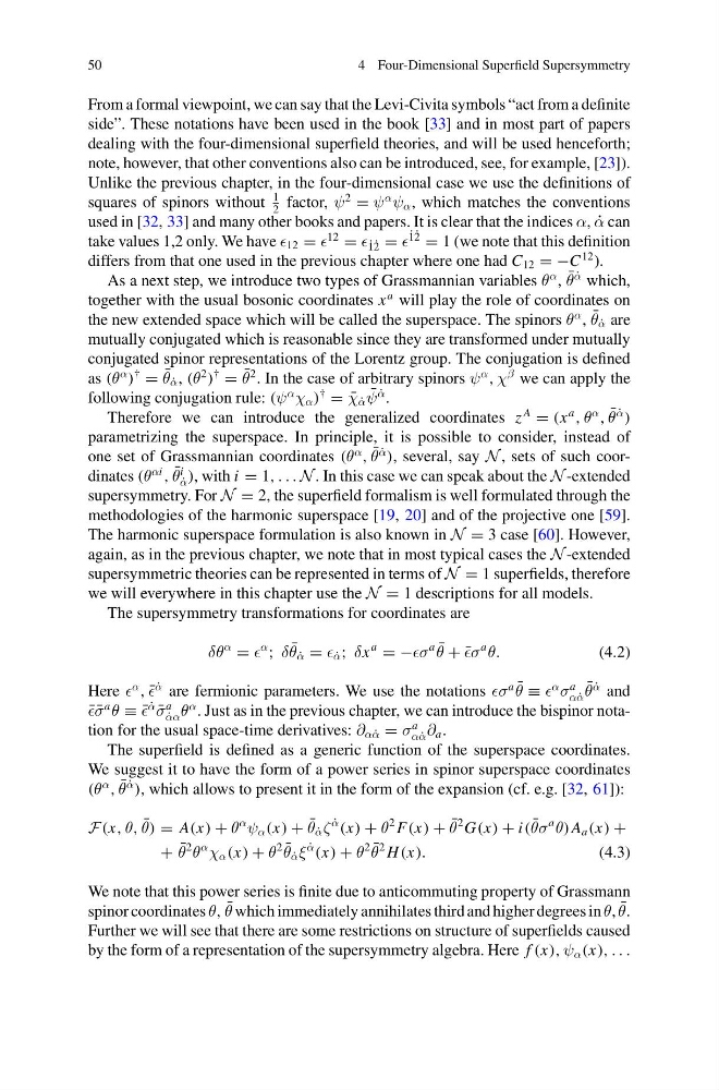
The supersymmetry transformations for coordinates are
δθ
α
=
α
; δ ¯
θ ˙
α = ˙
α ; δx
a
= −σ
a ¯
θ + ¯
σ
a
θ.
(4.2)
Here
α
, ¯
˙
α are fermionic parameters. We use the notations σ
a ¯
θ ≡
α
σ
a
α ˙
α
¯
θ
˙
α and
¯
¯
σ
a
θ ≡ ¯
˙
α
¯
σ
a
˙
αα θ
α . Just as in the previous chapter, we can introduce the bispinor notation for the usual space-time derivatives: ∂ α ˙
α = σ
a
α ˙
α ∂ a .
The superfield is defined as a generic function of the superspace coordinates.
We suggest it to have the form of a power series in spinor superspace coordinates
(θ
α
, ¯
θ
˙
α
), which allows to present it in the form of the expansion (cf. e.g. [32, 61]):
F(x, θ, ¯
θ) = A(x) + θ
α
ψ α (x) + ¯
θ ˙
α ζ
˙
α
(x) + θ
2 F(x) + ¯
θ
2 G(x) + i( ¯
θσ
a
θ)A a (x) +
+ ¯
θ
2
θ
α
χ α (x) + θ
2 ¯
θ ˙
α ξ
˙
α
(x) + θ
2 ¯
θ
2 H (x).
(4.3)
We note that this power series is finite due to anticommuting property of Grassmann
spinor coordinates θ, ¯
θ which immediately annihilates third and higher degrees in θ, ¯
θ.
Further we will see that there are some restrictions on structure of superfields caused
by the form of a representation of the supersymmetry algebra. Here f (x), ψ α (x), . . .
4 Four-Dimensional Superfield Supersymmetry
From a formal viewpoint, we can say that the Levi-Civita symbols “act from a definite
side”. These notations have been used in the book [33] and in most part of papers
dealing with the four-dimensional superfield theories, and will be used henceforth;
note, however, that other conventions also can be introduced, see, for example, [23]).
Unlike the previous chapter, in the four-dimensional case we use the definitions of
squares of spinors without
1
2
factor, ψ
2
= ψ
α
ψ α , which matches the conventions
used in [32, 33] and many other books and papers. It is clear that the indices α, ˙
α can
take values 1,2 only. We have 12 =
12
= ˙ 1 ˙
2 =
˙
1 ˙
2
= 1 (we note that this definition
differs from that one used in the previous chapter where one had C 12 = −C
12 ).
As a next step, we introduce two types of Grassmannian variables θ
α , ¯
θ
˙
α which,
together with the usual bosonic coordinates x
a will play the role of coordinates on
the new extended space which will be called the superspace. The spinors θ
α , ¯
θ ˙
α are
mutually conjugated which is reasonable since they are transformed under mutually
conjugated spinor representations of the Lorentz group. The conjugation is defined
as (θ
α
)
†
= ¯
θ ˙
α , (θ
2
)
†
= ¯
θ
2 . In the case of arbitrary spinors ψ
α
, χ
β we can apply the
following conjugation rule: (ψ
α
χ α )
†
= ¯
χ ˙
α
¯
ψ
˙
α .
Therefore we can introduce the generalized coordinates z
A
= (x
a
, θ
α
, ¯
θ
˙
α
)
parametrizing the superspace. In principle, it is possible to consider, instead of
one set of Grassmannian coordinates (θ
α
, ¯
θ
˙
α
), several, say N , sets of such coordinates (θ
αi
, ¯
θ
i
˙
α ), with i = 1, . . . N . In this case we can speak about the N -extended
supersymmetry. For N = 2, the superfield formalism is well formulated through the
methodologies of the harmonic superspace [19, 20] and of the projective one [59].
The harmonic superspace formulation is also known in N = 3 case [60]. However,
again, as in the previous chapter, we note that in most typical cases the N -extended
supersymmetric theories can be represented in terms of N = 1 superfields, therefore
we will everywhere in this chapter use the N = 1 descriptions for all models.
The supersymmetry transformations for coordinates are
δθ
α
=
α
; δ ¯
θ ˙
α = ˙
α ; δx
a
= −σ
a ¯
θ + ¯
σ
a
θ.
(4.2)
Here
α
, ¯
˙
α are fermionic parameters. We use the notations σ
a ¯
θ ≡
α
σ
a
α ˙
α
¯
θ
˙
α and
¯
¯
σ
a
θ ≡ ¯
˙
α
¯
σ
a
˙
αα θ
α . Just as in the previous chapter, we can introduce the bispinor notation for the usual space-time derivatives: ∂ α ˙
α = σ
a
α ˙
α ∂ a .
The superfield is defined as a generic function of the superspace coordinates.
We suggest it to have the form of a power series in spinor superspace coordinates
(θ
α
, ¯
θ
˙
α
), which allows to present it in the form of the expansion (cf. e.g. [32, 61]):
F(x, θ, ¯
θ) = A(x) + θ
α
ψ α (x) + ¯
θ ˙
α ζ
˙
α
(x) + θ
2 F(x) + ¯
θ
2 G(x) + i( ¯
θσ
a
θ)A a (x) +
+ ¯
θ
2
θ
α
χ α (x) + θ
2 ¯
θ ˙
α ξ
˙
α
(x) + θ
2 ¯
θ
2 H (x).
(4.3)
We note that this power series is finite due to anticommuting property of Grassmann
spinor coordinates θ, ¯
θ which immediately annihilates third and higher degrees in θ, ¯
θ.
Further we will see that there are some restrictions on structure of superfields caused
by the form of a representation of the supersymmetry algebra. Here f (x), ψ α (x), . . .