

38
3 Superfield Description of Three-Dimensional Supersymmetric Theories
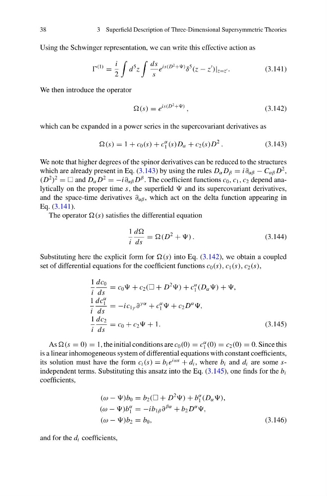
Using the Schwinger representation, we can write this effective action as
(1)
=
i
2
d
5 z
ds
s
e
is(D
2 +)
δ
5
(z − z
)| z=z .
(3.141)
We then introduce the operator
(s) = e
is(D
2 +)
,
(3.142)
which can be expanded in a power series in the supercovariant derivatives as
(s) = 1 + c 0 (s) + c
α
1 (s)D α + c 2 (s)D
2
.
(3.143)
We note that higher degrees of the spinor derivatives can be reduced to the structures
which are already present in Eq. (3.143) by using the rules D α D β = i∂ αβ − C αβ D
2 ,
(D
2
)
2
= and D α D
2
= −i∂ αβ D
β . The coefficient functions c 0 , c 1 , c 2 depend analytically on the proper time s, the superfield and its supercovariant derivatives,
and the space-time derivatives ∂ αβ , which act on the delta function appearing in
Eq. (3.141).
The operator (s) satisfies the differential equation
1
i
d
ds
= (D
2
+ ) .
(3.144)
Substituting here the explicit form for (s) into Eq. (3.142), we obtain a coupled
set of differential equations for the coefficient functions c 0 (s), c 1 (s), c 2 (s),
1
i
dc 0
ds
= c 0 + c 2 ( + D
2
) + c
α
1 (D α ) + ,
1
i
dc
α
1
ds
= −ic 1γ ∂
γ α
+ c
α
1 + c 2 D
α
,
1
i
dc 2
ds
= c 0 + c 2 + 1.
(3.145)
As (s = 0) = 1, the initial conditions are c 0 (0) = c
α
1 (0) = c 2 (0) = 0. Since this
is a linear inhomogeneous system of differential equations with constant coefficients,
its solution must have the form c i (s) = b i e
iωs
+ d i , where b i and d i are some sindependent terms. Substituting this ansatz into the Eq. (3.145), one finds for the b i
coefficients,
(ω − )b 0 = b 2 ( + D
2
) + b
α
1 (D α ),
(ω − )b
α
1 = −ib 1β ∂
βα
+ b 2 D
α
,
(ω − )b 2 = b 0 ,
(3.146)
and for the d i coefficients,
3 Superfield Description of Three-Dimensional Supersymmetric Theories
Using the Schwinger representation, we can write this effective action as
(1)
=
i
2
d
5 z
ds
s
e
is(D
2 +)
δ
5
(z − z
)| z=z .
(3.141)
We then introduce the operator
(s) = e
is(D
2 +)
,
(3.142)
which can be expanded in a power series in the supercovariant derivatives as
(s) = 1 + c 0 (s) + c
α
1 (s)D α + c 2 (s)D
2
.
(3.143)
We note that higher degrees of the spinor derivatives can be reduced to the structures
which are already present in Eq. (3.143) by using the rules D α D β = i∂ αβ − C αβ D
2 ,
(D
2
)
2
= and D α D
2
= −i∂ αβ D
β . The coefficient functions c 0 , c 1 , c 2 depend analytically on the proper time s, the superfield and its supercovariant derivatives,
and the space-time derivatives ∂ αβ , which act on the delta function appearing in
Eq. (3.141).
The operator (s) satisfies the differential equation
1
i
d
ds
= (D
2
+ ) .
(3.144)
Substituting here the explicit form for (s) into Eq. (3.142), we obtain a coupled
set of differential equations for the coefficient functions c 0 (s), c 1 (s), c 2 (s),
1
i
dc 0
ds
= c 0 + c 2 ( + D
2
) + c
α
1 (D α ) + ,
1
i
dc
α
1
ds
= −ic 1γ ∂
γ α
+ c
α
1 + c 2 D
α
,
1
i
dc 2
ds
= c 0 + c 2 + 1.
(3.145)
As (s = 0) = 1, the initial conditions are c 0 (0) = c
α
1 (0) = c 2 (0) = 0. Since this
is a linear inhomogeneous system of differential equations with constant coefficients,
its solution must have the form c i (s) = b i e
iωs
+ d i , where b i and d i are some sindependent terms. Substituting this ansatz into the Eq. (3.145), one finds for the b i
coefficients,
(ω − )b 0 = b 2 ( + D
2
) + b
α
1 (D α ),
(ω − )b
α
1 = −ib 1β ∂
βα
+ b 2 D
α
,
(ω − )b 2 = b 0 ,
(3.146)
and for the d i coefficients,