

34
3 Superfield Description of Three-Dimensional Supersymmetric Theories
e.g. [46]). It is sufficient to use only the standard condition for this superfield to be
slowly varying in the space-time, ∂ m = 0.
We will work with a loop expansion for the effective action ,
[] = S[] +
(1)
[] +
2
(2)
[] + . . . ,
(3.119)
for the Kählerian potential K ,
K (() = −V (() +
∞
L=1
L K L ((),
(3.120)
and similarly for F.
We start by considering the one-loop effective action in the form
(1)
=
i
2
Tr ln[D
2
− V
(()].
(3.121)
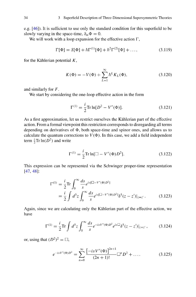
As a first approximation, let us restrict ourselves the Kählerian part of the effective
action. From a formal viewpoint this restriction corresponds to disregarding all terms
depending on derivatives of , both space-time and spinor ones, and allows us to
calculate the quantum corrections to V ((). In this case, we add a field independent
term
i
2
Tr ln(D
2
) and write
(1)
=
i
2
Tr ln[ − V
(()D
2
].
(3.122)
This expression can be represented via the Schwinger proper-time representation
[47, 48]:
(1)
=
i
2
Tr
∞
0
ds
s
e
is[−V
(()D
2 ]
=
i
2
d
5 z
∞
0
ds
s
e
is[−V
(()D
2 ]
δ
5
(z − z
)| z=z .
(3.123)
Again, since we are calculating only the Kählerian part of the effective action, we
have
(1)
=
i
2
Tr
d
5 z
∞
0
ds
s
e
−isV
(()D
2 e
is
δ
5
(z − z
)| z=z ,
(3.124)
or, using that (D
2
)
2
= ,
e
−isV
(()D
2 =
∞
n=0
−isV
(()
2n+1
(2n + 1)!
n D
2
+ . . . .
(3.125)
3 Superfield Description of Three-Dimensional Supersymmetric Theories
e.g. [46]). It is sufficient to use only the standard condition for this superfield to be
slowly varying in the space-time, ∂ m = 0.
We will work with a loop expansion for the effective action ,
[] = S[] +
(1)
[] +
2
(2)
[] + . . . ,
(3.119)
for the Kählerian potential K ,
K (() = −V (() +
∞
L=1
L K L ((),
(3.120)
and similarly for F.
We start by considering the one-loop effective action in the form
(1)
=
i
2
Tr ln[D
2
− V
(()].
(3.121)
As a first approximation, let us restrict ourselves the Kählerian part of the effective
action. From a formal viewpoint this restriction corresponds to disregarding all terms
depending on derivatives of , both space-time and spinor ones, and allows us to
calculate the quantum corrections to V ((). In this case, we add a field independent
term
i
2
Tr ln(D
2
) and write
(1)
=
i
2
Tr ln[ − V
(()D
2
].
(3.122)
This expression can be represented via the Schwinger proper-time representation
[47, 48]:
(1)
=
i
2
Tr
∞
0
ds
s
e
is[−V
(()D
2 ]
=
i
2
d
5 z
∞
0
ds
s
e
is[−V
(()D
2 ]
δ
5
(z − z
)| z=z .
(3.123)
Again, since we are calculating only the Kählerian part of the effective action, we
have
(1)
=
i
2
Tr
d
5 z
∞
0
ds
s
e
−isV
(()D
2 e
is
δ
5
(z − z
)| z=z ,
(3.124)
or, using that (D
2
)
2
= ,
e
−isV
(()D
2 =
∞
n=0
−isV
(()
2n+1
(2n + 1)!
n D
2
+ . . . .
(3.125)