

3.4 Quantum Description for the Superfield Models
29
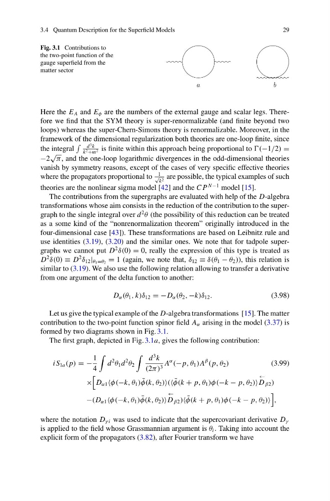
Fig. 3.1 Contributions to
the two-point function of the
gauge superfield from the
matter sector
a
b
Here the E A and E φ are the numbers of the external gauge and scalar legs. Therefore we find that the SYM theory is super-renormalizable (and finite beyond two
loops) whereas the super-Chern-Simons theory is renormalizable. Moreover, in the
framework of the dimensional regularization both theories are one-loop finite, since
the integral
d
3 k
k 2 +m 2 is finite within this approach being proportional to =
−2
√ π , and the one-loop logarithmic divergences in the odd-dimensional theories
vanish by symmetry reasons, except of the cases of very specific effective theories
where the propagators proportional to
1
√
k 2 are possible, the typical examples of such
theories are the nonlinear sigma model [42] and the C P
N −1 model [15].
The contributions from the supergraphs are evaluated with help of the D-algebra
transformations whose aim consists in the reduction of the contribution to the supergraph to the single integral over d
2
θ (the possibility of this reduction can be treated
as a some kind of the “nonrenormalization theorem” originally introduced in the
four-dimensional case [43]). These transformations are based on Leibnitz rule and
use identities (3.19), (3.20) and the similar ones. We note that for tadpole supergraphs we cannot put D
2
δ(0) = 0, really the expression of this type is treated as
D
2
δ(0) ≡ D
2
δ 12 | θ 1 =θ 2 = 1 (again, we note that, δ 12 ≡ δ(θ 1 − θ 2 )), this relation is
similar to (3.19). We also use the following relation allowing to transfer a derivative
from one argument of the delta function to another:
D α (θ 1 , k)δ 12 = −D α (θ 2 , −k)δ 12 .
(3.98)
Let us give the typical example of the D-algebra transformations [15]. The matter
contribution to the two-point function spinor field A α arising in the model (3.37) is
formed by two diagrams shown in Fig. 3.1.
The first graph, depicted in Fig. 3.1a, gives the following contribution:
i S 1a ( p) = −
1
4
d
2
θ 1 d
2
θ 2
d
3 k
(2π) 3 A
α
(− p, θ 1 )A
β
( p, θ 2 )
(3.99)
×
D α1 φ(−k, θ 1 ) ¯
φ(k, θ 2 ) ¯
φ(k + p, θ 1 )φ(−k − p, θ 2 )
←
D β2 )
−(D α1 φ(−k, θ 1 ) ¯
φ(k, θ 2 )
←
D β2 ) ¯
φ(k + p, θ 1 )φ(−k − p, θ 2 )
,
where the notation D γ i was used to indicate that the supercovariant derivative D γ
is applied to the field whose Grassmannian argument is θ i . Taking into account the
explicit form of the propagators (3.82), after Fourier transform we have
29
Fig. 3.1 Contributions to
the two-point function of the
gauge superfield from the
matter sector
a
b
Here the E A and E φ are the numbers of the external gauge and scalar legs. Therefore we find that the SYM theory is super-renormalizable (and finite beyond two
loops) whereas the super-Chern-Simons theory is renormalizable. Moreover, in the
framework of the dimensional regularization both theories are one-loop finite, since
the integral
d
3 k
k 2 +m 2 is finite within this approach being proportional to =
−2
√ π , and the one-loop logarithmic divergences in the odd-dimensional theories
vanish by symmetry reasons, except of the cases of very specific effective theories
where the propagators proportional to
1
√
k 2 are possible, the typical examples of such
theories are the nonlinear sigma model [42] and the C P
N −1 model [15].
The contributions from the supergraphs are evaluated with help of the D-algebra
transformations whose aim consists in the reduction of the contribution to the supergraph to the single integral over d
2
θ (the possibility of this reduction can be treated
as a some kind of the “nonrenormalization theorem” originally introduced in the
four-dimensional case [43]). These transformations are based on Leibnitz rule and
use identities (3.19), (3.20) and the similar ones. We note that for tadpole supergraphs we cannot put D
2
δ(0) = 0, really the expression of this type is treated as
D
2
δ(0) ≡ D
2
δ 12 | θ 1 =θ 2 = 1 (again, we note that, δ 12 ≡ δ(θ 1 − θ 2 )), this relation is
similar to (3.19). We also use the following relation allowing to transfer a derivative
from one argument of the delta function to another:
D α (θ 1 , k)δ 12 = −D α (θ 2 , −k)δ 12 .
(3.98)
Let us give the typical example of the D-algebra transformations [15]. The matter
contribution to the two-point function spinor field A α arising in the model (3.37) is
formed by two diagrams shown in Fig. 3.1.
The first graph, depicted in Fig. 3.1a, gives the following contribution:
i S 1a ( p) = −
1
4
d
2
θ 1 d
2
θ 2
d
3 k
(2π) 3 A
α
(− p, θ 1 )A
β
( p, θ 2 )
(3.99)
×
D α1 φ(−k, θ 1 ) ¯
φ(k, θ 2 ) ¯
φ(k + p, θ 1 )φ(−k − p, θ 2 )
←
D β2 )
−(D α1 φ(−k, θ 1 ) ¯
φ(k, θ 2 )
←
D β2 ) ¯
φ(k + p, θ 1 )φ(−k − p, θ 2 )
,
where the notation D γ i was used to indicate that the supercovariant derivative D γ
is applied to the field whose Grassmannian argument is θ i . Taking into account the
explicit form of the propagators (3.82), after Fourier transform we have