

4.8 The Wess-Zumino Model and a Problem of the Chiral Effective Potential
95
K
(1)
= −
1
32π 2 ¯
∞
¯
L 2
dt
t
1
0
due
−
t
4 (1−u
2 )
.
(4.177)
At L
2
→ 0 this integral tends to
K
(1)
= −
1
32π 2 ¯
log(μ
2 L
2
) −
1
32π 2 ¯
(log
¯
μ 2 − ξ),
(4.178)
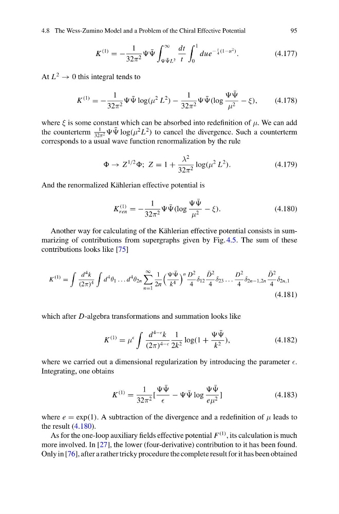
where ξ is some constant which can be absorbed into redefinition of μ. We can add
the counterterm
1
32π 2 ¯
log(μ
2 L
2
) to cancel the divergence. Such a counterterm
corresponds to a usual wave function renormalization by the rule
→ Z
1/2
; Z = 1 +
λ
2
32π 2 log(μ
2 L
2
).
(4.179)
And the renormalized Kählerian effective potential is
K
(1)
ren = −
1
32π 2 ¯
(log
¯
μ 2 − ξ).
(4.180)
Another way for calculating of the Kählerian effective potential consists in summarizing of contributions from supergraphs given by Fig. 4.5. The sum of these
contributions looks like [75]
K
(1) =
d 4 k
(2π) 4
d
4 θ 1 . . . d
4 θ 2n
∞
n=1
1
2n
¯
k 4
n D 2
4
δ 12
¯
D 2
4
δ 23 . . .
D 2
4
δ 2n−1,2n
¯
D 2
4
δ 2n,1
(4.181)
which after D-algebra transformations and summation looks like
K
(1)
= μ
d
4− k
(2π) 4−
1
2k 2 log(1 +
¯
k 2 ),
(4.182)
where we carried out a dimensional regularization by introducing the parameter .
Integrating, one obtains
K
(1)
=
1
32π 2 [
¯
− ¯
log
¯
eμ 2 ]
(4.183)
where e = exp(1). A subtraction of the divergence and a redefinition of μ leads to
the result (4.180).
As for the one-loop auxiliary fields effective potential F
(1) , its calculation is much
more involved. In [27], the lower (four-derivative) contribution to it has been found.
Only in [76], after a rather tricky procedure the complete result for it has been obtained
95
K
(1)
= −
1
32π 2 ¯
∞
¯
L 2
dt
t
1
0
due
−
t
4 (1−u
2 )
.
(4.177)
At L
2
→ 0 this integral tends to
K
(1)
= −
1
32π 2 ¯
log(μ
2 L
2
) −
1
32π 2 ¯
(log
¯
μ 2 − ξ),
(4.178)
where ξ is some constant which can be absorbed into redefinition of μ. We can add
the counterterm
1
32π 2 ¯
log(μ
2 L
2
) to cancel the divergence. Such a counterterm
corresponds to a usual wave function renormalization by the rule
→ Z
1/2
; Z = 1 +
λ
2
32π 2 log(μ
2 L
2
).
(4.179)
And the renormalized Kählerian effective potential is
K
(1)
ren = −
1
32π 2 ¯
(log
¯
μ 2 − ξ).
(4.180)
Another way for calculating of the Kählerian effective potential consists in summarizing of contributions from supergraphs given by Fig. 4.5. The sum of these
contributions looks like [75]
K
(1) =
d 4 k
(2π) 4
d
4 θ 1 . . . d
4 θ 2n
∞
n=1
1
2n
¯
k 4
n D 2
4
δ 12
¯
D 2
4
δ 23 . . .
D 2
4
δ 2n−1,2n
¯
D 2
4
δ 2n,1
(4.181)
which after D-algebra transformations and summation looks like
K
(1)
= μ
d
4− k
(2π) 4−
1
2k 2 log(1 +
¯
k 2 ),
(4.182)
where we carried out a dimensional regularization by introducing the parameter .
Integrating, one obtains
K
(1)
=
1
32π 2 [
¯
− ¯
log
¯
eμ 2 ]
(4.183)
where e = exp(1). A subtraction of the divergence and a redefinition of μ leads to
the result (4.180).
As for the one-loop auxiliary fields effective potential F
(1) , its calculation is much
more involved. In [27], the lower (four-derivative) contribution to it has been found.
Only in [76], after a rather tricky procedure the complete result for it has been obtained