

2.6 Analytical Properties of the Wave Functions
67
To get rid of the explicit r-dependence in Eq. (2.196), further approximations are
necessary [48,49]. Neglecting (k) in the Coulomb wave functions of the numerator
implies that their Wronskian becomes equal to 2i(k). Moreover, as u(k, r) is a
metastable state, it decreases exponentially along the real r-axis in the asymptotic
region. Thus, the integral in the denominator is almost equal to one when r is chosen
in the asymptotic region. Under these assumptions, valid for narrow resonances,
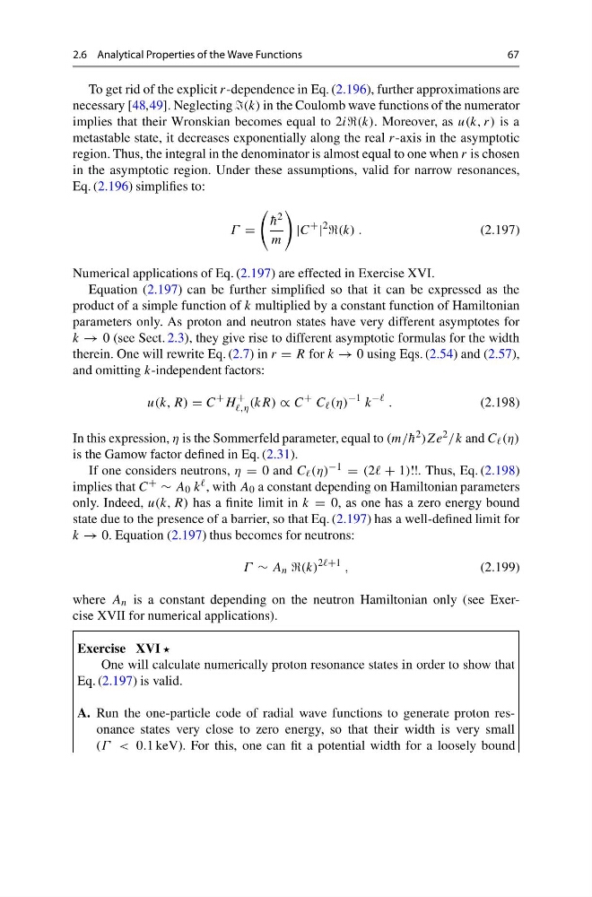
Eq. (2.196) simplifies to:
Γ =
¯
h 2
m
|C
+
|
2
(k) .
(2.197)
Numerical applications of Eq. (2.197) are effected in Exercise XVI.
Equation (2.197) can be further simplified so that it can be expressed as the
product of a simple function of k multiplied by a constant function of Hamiltonian
parameters only. As proton and neutron states have very different asymptotes for
k → 0 (see Sect. 2.3), they give rise to different asymptotic formulas for the width
therein. One will rewrite Eq. (2.7) in r = R for k → 0 using Eqs. (2.54) and (2.57),
and omitting k-independent factors:
u(k, R) = C
+ H
+
,η (kR) ∝ C
+ C (η)
−1 k
− .
(2.198)
In this expression, η is the Sommerfeld parameter, equal to (m/ ¯
h 2 )Ze 2 /k and C (η)
is the Gamow factor defined in Eq. (2.31).
If one considers neutrons, η = 0 and C (η) −1 = (2 + 1)!!. Thus, Eq. (2.198)
implies that C + ∼ A 0 k , with A 0 a constant depending on Hamiltonian parameters
only. Indeed, u(k, R) has a finite limit in k = 0, as one has a zero energy bound
state due to the presence of a barrier, so that Eq. (2.197) has a well-defined limit for
k → 0. Equation (2.197) thus becomes for neutrons:
Γ ∼ A n (k)
2 ,
(2.199)
where A n is a constant depending on the neutron Hamiltonian only (see Exercise XVII for numerical applications).
Exercise XVI
One will calculate numerically proton resonance states in order to show that
Eq. (2.197) is valid.
A. Run the one-particle code of radial wave functions to generate proton resonance states very close to zero energy, so that their width is very small
(Γ < 0.1 keV). For this, one can fit a potential width for a loosely bound
67
To get rid of the explicit r-dependence in Eq. (2.196), further approximations are
necessary [48,49]. Neglecting (k) in the Coulomb wave functions of the numerator
implies that their Wronskian becomes equal to 2i(k). Moreover, as u(k, r) is a
metastable state, it decreases exponentially along the real r-axis in the asymptotic
region. Thus, the integral in the denominator is almost equal to one when r is chosen
in the asymptotic region. Under these assumptions, valid for narrow resonances,
Eq. (2.196) simplifies to:
Γ =
¯
h 2
m
|C
+
|
2
(k) .
(2.197)
Numerical applications of Eq. (2.197) are effected in Exercise XVI.
Equation (2.197) can be further simplified so that it can be expressed as the
product of a simple function of k multiplied by a constant function of Hamiltonian
parameters only. As proton and neutron states have very different asymptotes for
k → 0 (see Sect. 2.3), they give rise to different asymptotic formulas for the width
therein. One will rewrite Eq. (2.7) in r = R for k → 0 using Eqs. (2.54) and (2.57),
and omitting k-independent factors:
u(k, R) = C
+ H
+
,η (kR) ∝ C
+ C (η)
−1 k
− .
(2.198)
In this expression, η is the Sommerfeld parameter, equal to (m/ ¯
h 2 )Ze 2 /k and C (η)
is the Gamow factor defined in Eq. (2.31).
If one considers neutrons, η = 0 and C (η) −1 = (2 + 1)!!. Thus, Eq. (2.198)
implies that C + ∼ A 0 k , with A 0 a constant depending on Hamiltonian parameters
only. Indeed, u(k, R) has a finite limit in k = 0, as one has a zero energy bound
state due to the presence of a barrier, so that Eq. (2.197) has a well-defined limit for
k → 0. Equation (2.197) thus becomes for neutrons:
Γ ∼ A n (k)
2 ,
(2.199)
where A n is a constant depending on the neutron Hamiltonian only (see Exercise XVII for numerical applications).
Exercise XVI
One will calculate numerically proton resonance states in order to show that
Eq. (2.197) is valid.
A. Run the one-particle code of radial wave functions to generate proton resonance states very close to zero energy, so that their width is very small
(Γ < 0.1 keV). For this, one can fit a potential width for a loosely bound