

2.6 Analytical Properties of the Wave Functions
51
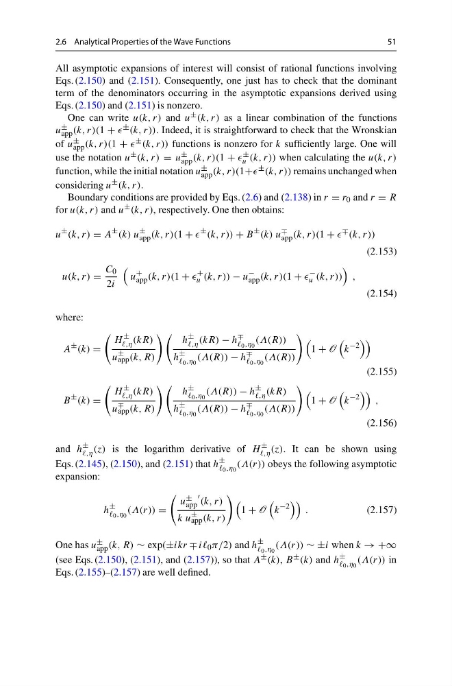
All asymptotic expansions of interest will consist of rational functions involving
Eqs. (2.150) and (2.151). Consequently, one just has to check that the dominant
term of the denominators occurring in the asymptotic expansions derived using
Eqs. (2.150) and (2.151) is nonzero.
One can write u(k, r) and u ± (k, r) as a linear combination of the functions
u ±
app (k, r)(1 + ± (k, r)). Indeed, it is straightforward to check that the Wronskian
of u ±
app (k, r)(1 + ± (k, r)) functions is nonzero for k sufficiently large. One will
use the notation u ± (k, r) = u ±
app (k, r)(1 + ±
u (k, r)) when calculating the u(k, r)
function, while the initial notation u ±
app (k, r)(1+ ± (k, r)) remains unchanged when
considering u ± (k, r).
Boundary conditions are provided by Eqs. (2.6) and (2.138) in r = r 0 and r = R
for u(k, r) and u ± (k, r), respectively. One then obtains:
u
± (k, r) = A
± (k) u
±
app (k, r)(1 +
± (k, r)) + B
± (k) u
∓
app (k, r)(1 +
∓ (k, r))
(2.153)
u(k, r) =
C 0
2i
u
+
app (k, r)(1 +
+
u (k, r)) − u
−
app (k, r)(1 +
−
u (k, r))
,
(2.154)
where:
A
± (k) =
H
±
,η (kR)
u
±
app (k, R)
h
±
,η (kR) − h
∓
0 ,η 0
(Λ(R))
h
±
0 ,η 0
(Λ(R)) − h
∓
0 ,η 0
(Λ(R))
1 + O
k
−2
(2.155)
B
± (k) =
H
±
,η (kR)
u
∓
app (k, R)
h
±
0 ,η 0
(Λ(R)) − h
±
,η (kR)
h
±
0 ,η 0
(Λ(R)) − h
∓
0 ,η 0
(Λ(R))
1 + O
k
−2
,
(2.156)
and h
±
,η (z) is the logarithm derivative of H
±
,η (z). It can be shown using
Eqs. (2.145), (2.150), and (2.151) that h
±
0 ,η 0
(Λ(r)) obeys the following asymptotic
expansion:
h
±
0 ,η 0
(Λ(r)) =
u ±
app
(k, r)
k u
±
app (k, r)
1 + O
k
−2
.
(2.157)
One has u ±
app (k, R) ∼ exp(±ikr ∓ ii 0 π/2) and h
±
0 ,η 0
(Λ(r)) ∼ ±i when k → +∞
(see Eqs. (2.150), (2.151), and (2.157)), so that A ± (k), B ± (k) and h
±
0 ,η 0
(Λ(r)) in
Eqs. (2.155)–(2.157) are well defined.
51
All asymptotic expansions of interest will consist of rational functions involving
Eqs. (2.150) and (2.151). Consequently, one just has to check that the dominant
term of the denominators occurring in the asymptotic expansions derived using
Eqs. (2.150) and (2.151) is nonzero.
One can write u(k, r) and u ± (k, r) as a linear combination of the functions
u ±
app (k, r)(1 + ± (k, r)). Indeed, it is straightforward to check that the Wronskian
of u ±
app (k, r)(1 + ± (k, r)) functions is nonzero for k sufficiently large. One will
use the notation u ± (k, r) = u ±
app (k, r)(1 + ±
u (k, r)) when calculating the u(k, r)
function, while the initial notation u ±
app (k, r)(1+ ± (k, r)) remains unchanged when
considering u ± (k, r).
Boundary conditions are provided by Eqs. (2.6) and (2.138) in r = r 0 and r = R
for u(k, r) and u ± (k, r), respectively. One then obtains:
u
± (k, r) = A
± (k) u
±
app (k, r)(1 +
± (k, r)) + B
± (k) u
∓
app (k, r)(1 +
∓ (k, r))
(2.153)
u(k, r) =
C 0
2i
u
+
app (k, r)(1 +
+
u (k, r)) − u
−
app (k, r)(1 +
−
u (k, r))
,
(2.154)
where:
A
± (k) =
H
±
,η (kR)
u
±
app (k, R)
h
±
,η (kR) − h
∓
0 ,η 0
(Λ(R))
h
±
0 ,η 0
(Λ(R)) − h
∓
0 ,η 0
(Λ(R))
1 + O
k
−2
(2.155)
B
± (k) =
H
±
,η (kR)
u
∓
app (k, R)
h
±
0 ,η 0
(Λ(R)) − h
±
,η (kR)
h
±
0 ,η 0
(Λ(R)) − h
∓
0 ,η 0
(Λ(R))
1 + O
k
−2
,
(2.156)
and h
±
,η (z) is the logarithm derivative of H
±
,η (z). It can be shown using
Eqs. (2.145), (2.150), and (2.151) that h
±
0 ,η 0
(Λ(r)) obeys the following asymptotic
expansion:
h
±
0 ,η 0
(Λ(r)) =
u ±
app
(k, r)
k u
±
app (k, r)
1 + O
k
−2
.
(2.157)
One has u ±
app (k, R) ∼ exp(±ikr ∓ ii 0 π/2) and h
±
0 ,η 0
(Λ(r)) ∼ ±i when k → +∞
(see Eqs. (2.150), (2.151), and (2.157)), so that A ± (k), B ± (k) and h
±
0 ,η 0
(Λ(r)) in
Eqs. (2.155)–(2.157) are well defined.