

50
2 The Discrete Spectrum and the Continuum
properties of WKB approximation and from the fact that the functions entering
Eq. (2.145) are bounded on the real k-axis.
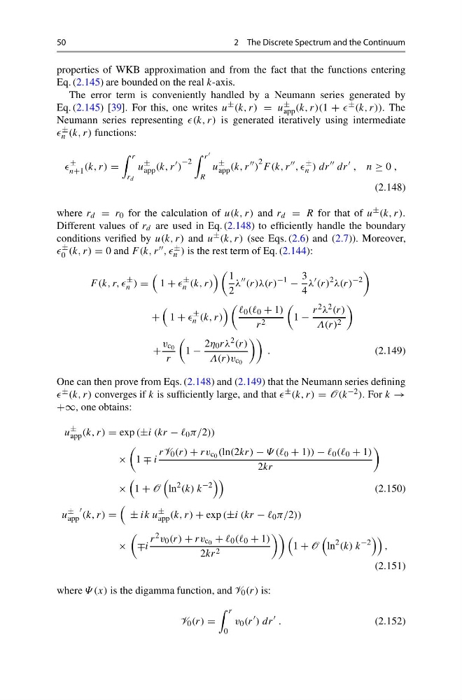
The error term is conveniently handled by a Neumann series generated by
Eq. (2.145) [39]. For this, one writes u ± (k, r) = u ±
app (k, r)(1 + ± (k, r)). The
Neumann series representing (k, r) is generated iteratively using intermediate
±
n (k, r) functions:
±
n+1 (k, r) =
r
r d
u
±
app (k, r
)
−2
r
R
u
±
app (k, r
)
2 F (k, r
, ,
±
n ) dr
dr
, n ≥ 0 ,
(2.148)
where r d = r 0 for the calculation of u(k, r) and r d = R for that of u ± (k, r).
Different values of r d are used in Eq. (2.148) to efficiently handle the boundary
conditions verified by u(k, r) and u ± (k, r) (see Eqs. (2.6) and (2.7)). Moreover,
±
0 (k, r) = 0 and F (k, r , , ±
n ) is the rest term of Eq. (2.144):
F (k, r, ,
±
n ) =
1 +
±
n (k, r)
1
2
λ
(r)λ(r)
−1
−
3
4
λ
(r)
2 λ(r)
−2
+
1 +
±
n (k, r)
0 (( 0 + 1)
r 2
1 −
r 2 λ 2 (r)
Λ(r) 2
+
v c 0
r
1 −
2η 0 rλ 2 (r)
Λ(r)v c 0
.
(2.149)
One can then prove from Eqs. (2.148) and (2.149) that the Neumann series defining
± (k, r) converges if k is sufficiently large, and that ± (k, r) = O(k −2 ). For k →
+∞, one obtains:
u
±
app (k, r) = exp (±i (kr − 0 π/2))
×
1 ∓ i
rV 0 (r) + rv c 0 (ln(2kr) − Ψ (( 0 + 1)) − 0 (( 0 + 1)
2kr
×
1 + O
ln
2 (k) k
−2
(2.150)
u
±
app
(k, r) =
± ik u
±
app (k, r) + exp (±i (kr − 0 π/2))
×
∓i
r 2 v 0 (r) + rv c 0 + 0 (( 0 + 1)
2kr 2
1 + O
ln
2 (k) k
−2
,
(2.151)
where Ψ (x) is the digamma function, and V 0 (r) is:
V 0 (r) =
r
0
v 0 (r
) dr
.
(2.152)
2 The Discrete Spectrum and the Continuum
properties of WKB approximation and from the fact that the functions entering
Eq. (2.145) are bounded on the real k-axis.
The error term is conveniently handled by a Neumann series generated by
Eq. (2.145) [39]. For this, one writes u ± (k, r) = u ±
app (k, r)(1 + ± (k, r)). The
Neumann series representing (k, r) is generated iteratively using intermediate
±
n (k, r) functions:
±
n+1 (k, r) =
r
r d
u
±
app (k, r
)
−2
r
R
u
±
app (k, r
)
2 F (k, r
, ,
±
n ) dr
dr
, n ≥ 0 ,
(2.148)
where r d = r 0 for the calculation of u(k, r) and r d = R for that of u ± (k, r).
Different values of r d are used in Eq. (2.148) to efficiently handle the boundary
conditions verified by u(k, r) and u ± (k, r) (see Eqs. (2.6) and (2.7)). Moreover,
±
0 (k, r) = 0 and F (k, r , , ±
n ) is the rest term of Eq. (2.144):
F (k, r, ,
±
n ) =
1 +
±
n (k, r)
1
2
λ
(r)λ(r)
−1
−
3
4
λ
(r)
2 λ(r)
−2
+
1 +
±
n (k, r)
0 (( 0 + 1)
r 2
1 −
r 2 λ 2 (r)
Λ(r) 2
+
v c 0
r
1 −
2η 0 rλ 2 (r)
Λ(r)v c 0
.
(2.149)
One can then prove from Eqs. (2.148) and (2.149) that the Neumann series defining
± (k, r) converges if k is sufficiently large, and that ± (k, r) = O(k −2 ). For k →
+∞, one obtains:
u
±
app (k, r) = exp (±i (kr − 0 π/2))
×
1 ∓ i
rV 0 (r) + rv c 0 (ln(2kr) − Ψ (( 0 + 1)) − 0 (( 0 + 1)
2kr
×
1 + O
ln
2 (k) k
−2
(2.150)
u
±
app
(k, r) =
± ik u
±
app (k, r) + exp (±i (kr − 0 π/2))
×
∓i
r 2 v 0 (r) + rv c 0 + 0 (( 0 + 1)
2kr 2
1 + O
ln
2 (k) k
−2
,
(2.151)
where Ψ (x) is the digamma function, and V 0 (r) is:
V 0 (r) =
r
0
v 0 (r
) dr
.
(2.152)