

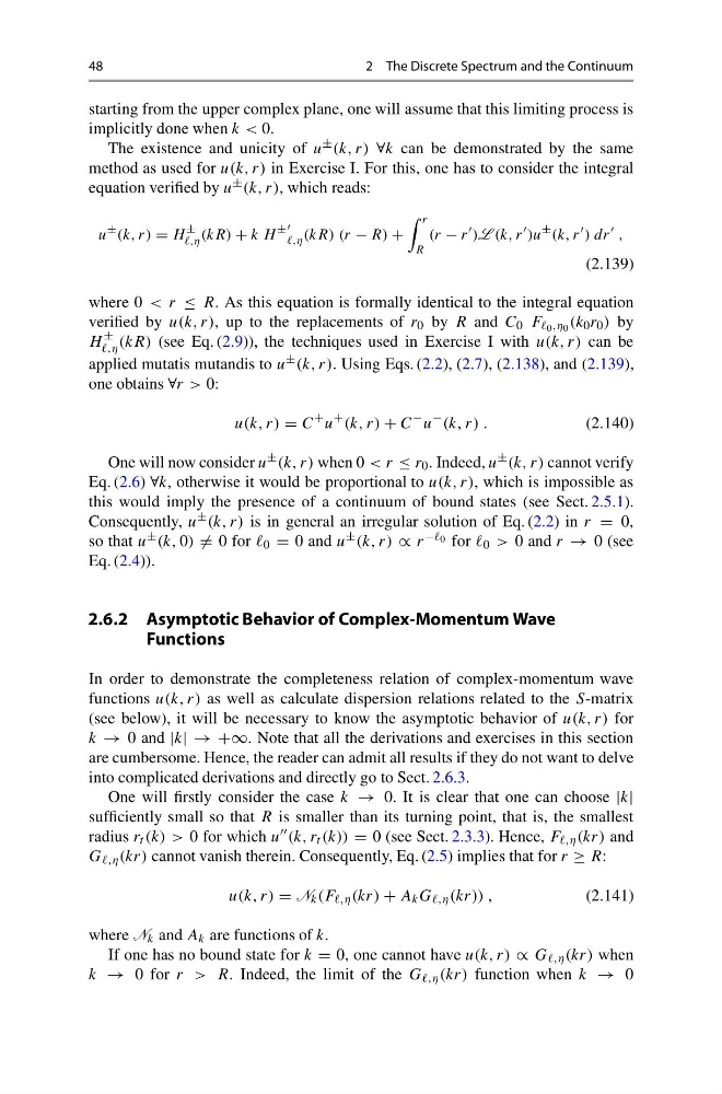
48
2 The Discrete Spectrum and the Continuum
starting from the upper complex plane, one will assume that this limiting process is
implicitly done when k < 0.
The existence and unicity of u ± (k, r) ∀k can be demonstrated by the same
method as used for u(k, r) in Exercise I. For this, one has to consider the integral
equation verified by u ± (k, r), which reads:
u
± (k, r) = H
±
,η (kR) + k H
±
,η (kR) (r − R) +
r
R
(r − r
)L (k, r
)u
± (k, r
) dr
,
(2.139)
where 0 < r ≤ R. As this equation is formally identical to the integral equation
verified by u(k, r), up to the replacements of r 0 by R and C 0 F 0 ,η 0 (k 0 r 0 ) by
H
±
,η (kR) (see Eq. (2.9)), the techniques used in Exercise I with u(k, r) can be
applied mutatis mutandis to u ± (k, r). Using Eqs. (2.2), (2.7), (2.138), and (2.139),
one obtains ∀r > 0:
u(k, r) = C
+ u
+ (k, r) + C
− u
− (k, r) .
(2.140)
One will now consider u ± (k, r) when 0 < r ≤ r 0 . Indeed, u ± (k, r) cannot verify
Eq. (2.6) ∀k, otherwise it would be proportional to u(k, r), which is impossible as
this would imply the presence of a continuum of bound states (see Sect. 2.5.1).
Consequently, u ± (k, r) is in general an irregular solution of Eq. (2.2) in r = 0,
so that u ± (k, 0) = 0 for 0 = 0 and u ± (k, r) ∝ r − 0 for 0 > 0 and r → 0 (see
Eq. (2.4)).
2.6.2 Asymptotic Behavior of Complex-Momentum Wave
Functions
In order to demonstrate the completeness relation of complex-momentum wave
functions u(k, r) as well as calculate dispersion relations related to the S-matrix
(see below), it will be necessary to know the asymptotic behavior of u(k, r) for
k → 0 and |k| → +∞. Note that all the derivations and exercises in this section
are cumbersome. Hence, the reader can admit all results if they do not want to delve
into complicated derivations and directly go to Sect. 2.6.3.
One will firstly consider the case k → 0. It is clear that one can choose |k|
sufficiently small so that R is smaller than its turning point, that is, the smallest
radius r t (k) > 0 for which u (k, r t (k)) = 0 (see Sect. 2.3.3). Hence, F ,η (kr) and
G ,η (kr) cannot vanish therein. Consequently, Eq. (2.5) implies that for r ≥ R:
u(k, r) = N k (F ,η (kr) + A k G ,η (kr)) ,
(2.141)
where N k and A k are functions of k.
If one has no bound state for k = 0, one cannot have u(k, r) ∝ G ,η (kr) when
k → 0 for r > R. Indeed, the limit of the G ,η (kr) function when k → 0
2 The Discrete Spectrum and the Continuum
starting from the upper complex plane, one will assume that this limiting process is
implicitly done when k < 0.
The existence and unicity of u ± (k, r) ∀k can be demonstrated by the same
method as used for u(k, r) in Exercise I. For this, one has to consider the integral
equation verified by u ± (k, r), which reads:
u
± (k, r) = H
±
,η (kR) + k H
±
,η (kR) (r − R) +
r
R
(r − r
)L (k, r
)u
± (k, r
) dr
,
(2.139)
where 0 < r ≤ R. As this equation is formally identical to the integral equation
verified by u(k, r), up to the replacements of r 0 by R and C 0 F 0 ,η 0 (k 0 r 0 ) by
H
±
,η (kR) (see Eq. (2.9)), the techniques used in Exercise I with u(k, r) can be
applied mutatis mutandis to u ± (k, r). Using Eqs. (2.2), (2.7), (2.138), and (2.139),
one obtains ∀r > 0:
u(k, r) = C
+ u
+ (k, r) + C
− u
− (k, r) .
(2.140)
One will now consider u ± (k, r) when 0 < r ≤ r 0 . Indeed, u ± (k, r) cannot verify
Eq. (2.6) ∀k, otherwise it would be proportional to u(k, r), which is impossible as
this would imply the presence of a continuum of bound states (see Sect. 2.5.1).
Consequently, u ± (k, r) is in general an irregular solution of Eq. (2.2) in r = 0,
so that u ± (k, 0) = 0 for 0 = 0 and u ± (k, r) ∝ r − 0 for 0 > 0 and r → 0 (see
Eq. (2.4)).
2.6.2 Asymptotic Behavior of Complex-Momentum Wave
Functions
In order to demonstrate the completeness relation of complex-momentum wave
functions u(k, r) as well as calculate dispersion relations related to the S-matrix
(see below), it will be necessary to know the asymptotic behavior of u(k, r) for
k → 0 and |k| → +∞. Note that all the derivations and exercises in this section
are cumbersome. Hence, the reader can admit all results if they do not want to delve
into complicated derivations and directly go to Sect. 2.6.3.
One will firstly consider the case k → 0. It is clear that one can choose |k|
sufficiently small so that R is smaller than its turning point, that is, the smallest
radius r t (k) > 0 for which u (k, r t (k)) = 0 (see Sect. 2.3.3). Hence, F ,η (kr) and
G ,η (kr) cannot vanish therein. Consequently, Eq. (2.5) implies that for r ≥ R:
u(k, r) = N k (F ,η (kr) + A k G ,η (kr)) ,
(2.141)
where N k and A k are functions of k.
If one has no bound state for k = 0, one cannot have u(k, r) ∝ G ,η (kr) when
k → 0 for r > R. Indeed, the limit of the G ,η (kr) function when k → 0