

34
2 The Discrete Spectrum and the Continuum
and y 0 = 1 as a starting point. As y ∼ 1, x n → x and y n → y rapidly for
n → +∞. Added to that, 1 − y 2 can be precisely evaluated with this algorithm,
because 1 − y
2
=
4e −2x
(1 + e −2x ) 2 , which is clearly devoid of numerical inaccuracy
when y ∼ 1.
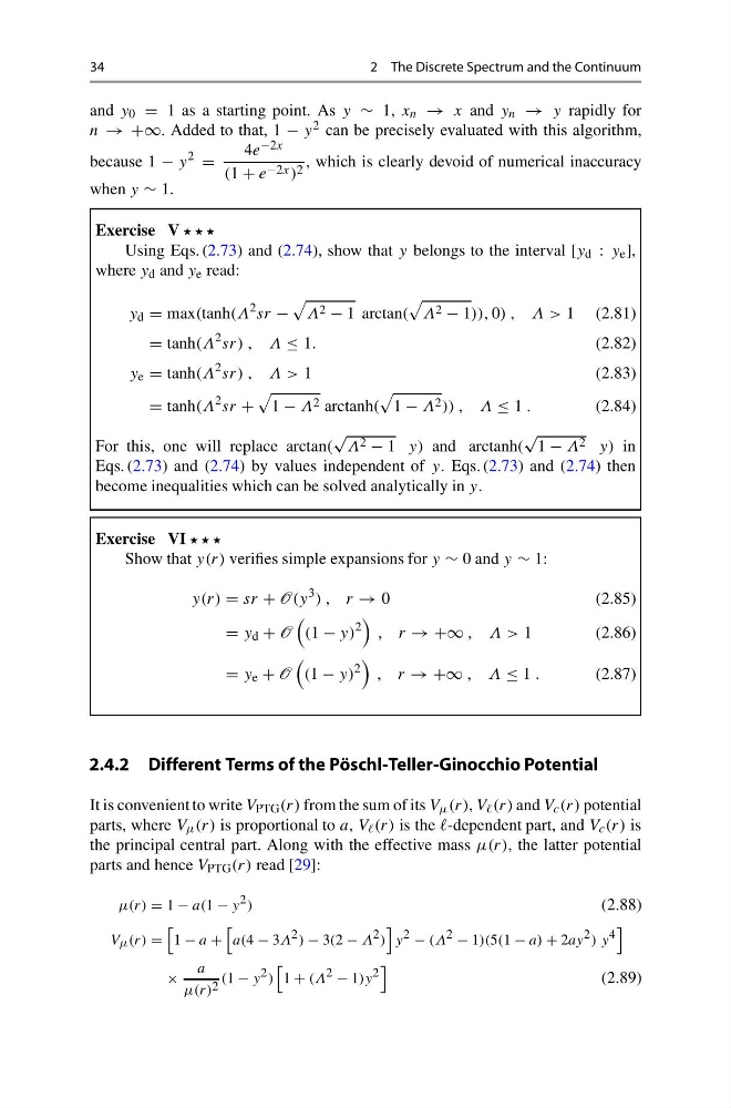
Exercise V
Using Eqs. (2.73) and (2.74), show that y belongs to the interval [y d : y e ],
where y d and y e read:
y d = max(tanh(Λ
2 sr −
Λ 2 − 1 arctan(
Λ 2 − 1)), 0) , Λ > 1 (2.81)
= tanh(Λ
2 sr) , Λ ≤ 1.
(2.82)
y e = tanh(Λ
2 sr) , Λ > 1
(2.83)
= tanh(Λ
2 sr +
1 − Λ 2 arctanh(
1 − Λ 2 )) , Λ ≤ 1 .
(2.84)
For this, one will replace arctan(
√
Λ 2 − 1 y) and arctanh(
√
1 − Λ 2 y) in
Eqs. (2.73) and (2.74) by values independent of y. Eqs. (2.73) and (2.74) then
become inequalities which can be solved analytically in y.
Exercise VI
Show that y(r) verifies simple expansions for y ∼ 0 and y ∼ 1:
y(r) = sr + O(y
3 ) , r → 0
(2.85)
= y d + O
(1 − y)
2
, r → +∞ , Λ > 1
(2.86)
= y e + O
(1 − y)
2
, r → +∞ , Λ ≤ 1 .
(2.87)
2.4.2 Different Terms of the Pöschl-Teller-Ginocchio Potential
It is convenient to write V PTG (r) from the sum of its V μ (r), V (r) and V c (r) potential
parts, where V μ (r) is proportional to a, V (r) is the -dependent part, and V c (r) is
the principal central part. Along with the effective mass μ(r), the latter potential
parts and hence V PTG (r) read [29]:
μ(r) = 1 − a(1 − y 2 )
(2.88)
V μ (r) =
1 − a +
a(4 − 3Λ 2 ) − 3(2 − Λ 2 )
y 2 − (Λ 2 − 1)(5(1 − a) + 2ay 2 ) y 4
×
a
μ(r) 2 (1 − y 2 )
1 + (Λ 2 − 1)y 2
(2.89)
2 The Discrete Spectrum and the Continuum
and y 0 = 1 as a starting point. As y ∼ 1, x n → x and y n → y rapidly for
n → +∞. Added to that, 1 − y 2 can be precisely evaluated with this algorithm,
because 1 − y
2
=
4e −2x
(1 + e −2x ) 2 , which is clearly devoid of numerical inaccuracy
when y ∼ 1.
Exercise V
Using Eqs. (2.73) and (2.74), show that y belongs to the interval [y d : y e ],
where y d and y e read:
y d = max(tanh(Λ
2 sr −
Λ 2 − 1 arctan(
Λ 2 − 1)), 0) , Λ > 1 (2.81)
= tanh(Λ
2 sr) , Λ ≤ 1.
(2.82)
y e = tanh(Λ
2 sr) , Λ > 1
(2.83)
= tanh(Λ
2 sr +
1 − Λ 2 arctanh(
1 − Λ 2 )) , Λ ≤ 1 .
(2.84)
For this, one will replace arctan(
√
Λ 2 − 1 y) and arctanh(
√
1 − Λ 2 y) in
Eqs. (2.73) and (2.74) by values independent of y. Eqs. (2.73) and (2.74) then
become inequalities which can be solved analytically in y.
Exercise VI
Show that y(r) verifies simple expansions for y ∼ 0 and y ∼ 1:
y(r) = sr + O(y
3 ) , r → 0
(2.85)
= y d + O
(1 − y)
2
, r → +∞ , Λ > 1
(2.86)
= y e + O
(1 − y)
2
, r → +∞ , Λ ≤ 1 .
(2.87)
2.4.2 Different Terms of the Pöschl-Teller-Ginocchio Potential
It is convenient to write V PTG (r) from the sum of its V μ (r), V (r) and V c (r) potential
parts, where V μ (r) is proportional to a, V (r) is the -dependent part, and V c (r) is
the principal central part. Along with the effective mass μ(r), the latter potential
parts and hence V PTG (r) read [29]:
μ(r) = 1 − a(1 − y 2 )
(2.88)
V μ (r) =
1 − a +
a(4 − 3Λ 2 ) − 3(2 − Λ 2 )
y 2 − (Λ 2 − 1)(5(1 − a) + 2ay 2 ) y 4
×
a
μ(r) 2 (1 − y 2 )
1 + (Λ 2 − 1)y 2
(2.89)