

30
2 The Discrete Spectrum and the Continuum
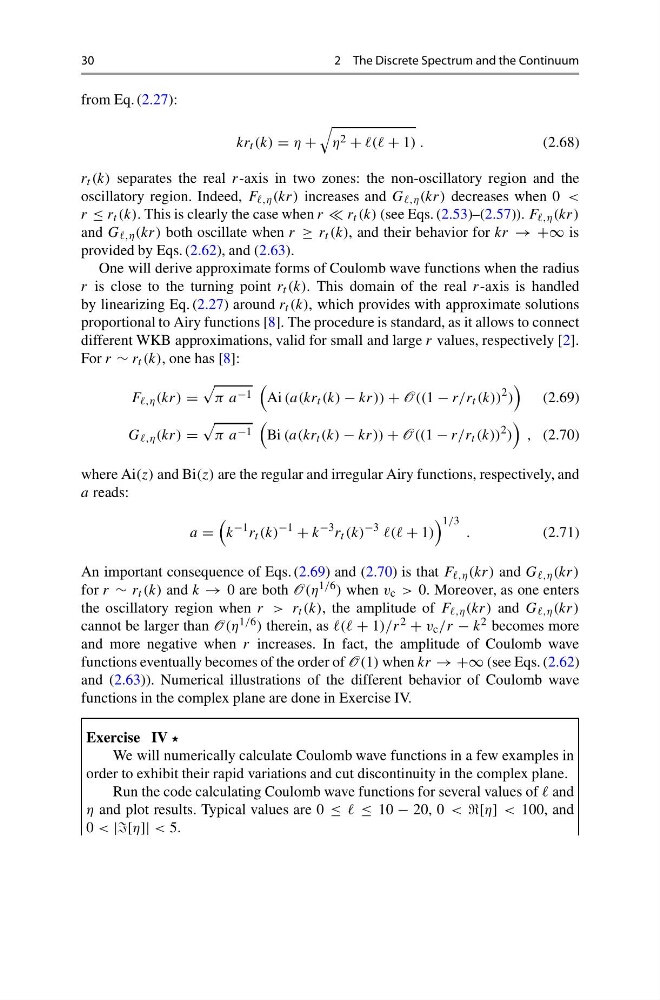
from Eq. (2.27):
kr t (k) = η +
η 2 + + 1) .
(2.68)
r t (k) separates the real r-axis in two zones: the non-oscillatory region and the
oscillatory region. Indeed, F ,η (kr) increases and G ,η (kr) decreases when 0 <
r ≤ r t (k). This is clearly the case when r r t (k) (see Eqs. (2.53)–(2.57)). F ,η (kr)
and G ,η (kr) both oscillate when r ≥ r t (k), and their behavior for kr → +∞ is
provided by Eqs. (2.62), and (2.63).
One will derive approximate forms of Coulomb wave functions when the radius
r is close to the turning point r t (k). This domain of the real r-axis is handled
by linearizing Eq. (2.27) around r t (k), which provides with approximate solutions
proportional to Airy functions [8]. The procedure is standard, as it allows to connect
different WKB approximations, valid for small and large r values, respectively [2].
For r ∼ r t (k), one has [8]:
F ,η (kr) =
π a −1
Ai (a(kr t (k) − kr)) + O((1 − r/r t (k))
2 )
(2.69)
G ,η (kr) =
π a −1
Bi (a(kr t (k) − kr)) + O((1 − r/r t (k))
2 )
, (2.70)
where Ai(z) and Bi(z) are the regular and irregular Airy functions, respectively, and
a reads:
a =
k
−1 r t (k)
−1
+ k
−3 r t (k)
−3 + 1)
1/3
.
(2.71)
An important consequence of Eqs. (2.69) and (2.70) is that F ,η (kr) and G ,η (kr)
for r ∼ r t (k) and k → 0 are both O(η 1/6 ) when v c > 0. Moreover, as one enters
the oscillatory region when r > r t (k), the amplitude of F ,η (kr) and G ,η (kr)
cannot be larger than O(η 1/6 ) therein, as + 1)/r 2 + v c /r − k 2 becomes more
and more negative when r increases. In fact, the amplitude of Coulomb wave
functions eventually becomes of the order of O(1) when kr → +∞ (see Eqs. (2.62)
and (2.63)). Numerical illustrations of the different behavior of Coulomb wave
functions in the complex plane are done in Exercise IV.
Exercise IV
We will numerically calculate Coulomb wave functions in a few examples in
order to exhibit their rapid variations and cut discontinuity in the complex plane.
Run the code calculating Coulomb wave functions for several values of and
η and plot results. Typical values are 0 ≤ ≤ 10 − 20, 0 < < 100, and
0 < ||[η]| < 5.
2 The Discrete Spectrum and the Continuum
from Eq. (2.27):
kr t (k) = η +
η 2 + + 1) .
(2.68)
r t (k) separates the real r-axis in two zones: the non-oscillatory region and the
oscillatory region. Indeed, F ,η (kr) increases and G ,η (kr) decreases when 0 <
r ≤ r t (k). This is clearly the case when r r t (k) (see Eqs. (2.53)–(2.57)). F ,η (kr)
and G ,η (kr) both oscillate when r ≥ r t (k), and their behavior for kr → +∞ is
provided by Eqs. (2.62), and (2.63).
One will derive approximate forms of Coulomb wave functions when the radius
r is close to the turning point r t (k). This domain of the real r-axis is handled
by linearizing Eq. (2.27) around r t (k), which provides with approximate solutions
proportional to Airy functions [8]. The procedure is standard, as it allows to connect
different WKB approximations, valid for small and large r values, respectively [2].
For r ∼ r t (k), one has [8]:
F ,η (kr) =
π a −1
Ai (a(kr t (k) − kr)) + O((1 − r/r t (k))
2 )
(2.69)
G ,η (kr) =
π a −1
Bi (a(kr t (k) − kr)) + O((1 − r/r t (k))
2 )
, (2.70)
where Ai(z) and Bi(z) are the regular and irregular Airy functions, respectively, and
a reads:
a =
k
−1 r t (k)
−1
+ k
−3 r t (k)
−3 + 1)
1/3
.
(2.71)
An important consequence of Eqs. (2.69) and (2.70) is that F ,η (kr) and G ,η (kr)
for r ∼ r t (k) and k → 0 are both O(η 1/6 ) when v c > 0. Moreover, as one enters
the oscillatory region when r > r t (k), the amplitude of F ,η (kr) and G ,η (kr)
cannot be larger than O(η 1/6 ) therein, as + 1)/r 2 + v c /r − k 2 becomes more
and more negative when r increases. In fact, the amplitude of Coulomb wave
functions eventually becomes of the order of O(1) when kr → +∞ (see Eqs. (2.62)
and (2.63)). Numerical illustrations of the different behavior of Coulomb wave
functions in the complex plane are done in Exercise IV.
Exercise IV
We will numerically calculate Coulomb wave functions in a few examples in
order to exhibit their rapid variations and cut discontinuity in the complex plane.
Run the code calculating Coulomb wave functions for several values of and
η and plot results. Typical values are 0 ≤ ≤ 10 − 20, 0 < < 100, and
0 < ||[η]| < 5.