

2.3 Coulomb Potential and Coulomb Wave Functions
27
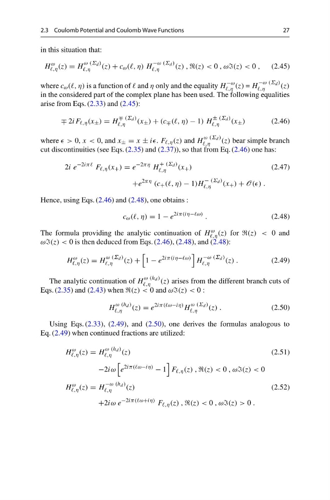
in this situation that:
H
ω
,η (z) = H
ω (Σ d )
,η
(z) + c ω ((, η) H
−ω (Σ d )
,η
(z) , (z) < 0 , ω(z) < 0 , (2.45)
where c ω ((, η) is a function of and η only and the equality H
−ω
,η (z) = H
−ω (Σ d )
,η
(z)
in the considered part of the complex plane has been used. The following equalities
arise from Eqs. (2.33) and (2.45):
∓ 2iF ,η (x ± ) = H
∓ (Σ d )
,η
(x ± ) + (c ∓ ((, η) − 1) H
± (Σ d )
,η
(x ± )
(2.46)
where > 0, x < 0, and x ± = x ± ii. F ,η (z) and H
ω (Σ d )
,η
(z) bear simple branch
cut discontinuities (see Eqs. (2.35) and (2.37)), so that from Eq. (2.46) one has:
2i e
−2iππ F ,η (x + ) = e
−2πη H
+ (Σ d )
,η
(x + )
(2.47)
+e
2πη (c + ((, η) − 1)H
− (Σ d )
,η
(x + ) + O(() .
Hence, using Eqs. (2.46) and (2.48), one obtains :
c ω ((, η) = 1 − e
2iπ(iη− .
(2.48)
The formula providing the analytic continuation of H ω
,η (z) for (z) < 0 and
ω(z) < 0 is then deduced from Eqs. (2.46), (2.48), and (2.48):
H
ω
,η (z) = H
ω (Σ d )
,η
(z) +
1 − e
2iπ(iη−
H
−ω (Σ d )
,η
(z) .
(2.49)
The analytic continuation of H
ω (h d )
,η
(z) arises from the different branch cuts of
Eqs. (2.35) and (2.43) when (z) < 0 and ω(z) < 0 :
H
ω (h d )
,η
(z) = e
2iπ((ω−iη) H
ω (Σ d )
,η
(z) .
(2.50)
Using Eqs. (2.33), (2.49), and (2.50), one derives the formulas analogous to
Eq. (2.49) when continued fractions are utilized:
H
ω
,η (z) = H
ω (h d )
,η
(z)
(2.51)
−2iω
e
2iπ((ω−iη)
− 1
F ,η (z) , (z) < 0 , ω(z) < 0
H
ω
,η (z) = H
−ω (h d )
,η
(z)
(2.52)
+2iω e
−2iπ((ω+iη) F ,η (z) , (z) < 0 , ω(z) > 0 .
27
in this situation that:
H
ω
,η (z) = H
ω (Σ d )
,η
(z) + c ω ((, η) H
−ω (Σ d )
,η
(z) , (z) < 0 , ω(z) < 0 , (2.45)
where c ω ((, η) is a function of and η only and the equality H
−ω
,η (z) = H
−ω (Σ d )
,η
(z)
in the considered part of the complex plane has been used. The following equalities
arise from Eqs. (2.33) and (2.45):
∓ 2iF ,η (x ± ) = H
∓ (Σ d )
,η
(x ± ) + (c ∓ ((, η) − 1) H
± (Σ d )
,η
(x ± )
(2.46)
where > 0, x < 0, and x ± = x ± ii. F ,η (z) and H
ω (Σ d )
,η
(z) bear simple branch
cut discontinuities (see Eqs. (2.35) and (2.37)), so that from Eq. (2.46) one has:
2i e
−2iππ F ,η (x + ) = e
−2πη H
+ (Σ d )
,η
(x + )
(2.47)
+e
2πη (c + ((, η) − 1)H
− (Σ d )
,η
(x + ) + O(() .
Hence, using Eqs. (2.46) and (2.48), one obtains :
c ω ((, η) = 1 − e
2iπ(iη− .
(2.48)
The formula providing the analytic continuation of H ω
,η (z) for (z) < 0 and
ω(z) < 0 is then deduced from Eqs. (2.46), (2.48), and (2.48):
H
ω
,η (z) = H
ω (Σ d )
,η
(z) +
1 − e
2iπ(iη−
H
−ω (Σ d )
,η
(z) .
(2.49)
The analytic continuation of H
ω (h d )
,η
(z) arises from the different branch cuts of
Eqs. (2.35) and (2.43) when (z) < 0 and ω(z) < 0 :
H
ω (h d )
,η
(z) = e
2iπ((ω−iη) H
ω (Σ d )
,η
(z) .
(2.50)
Using Eqs. (2.33), (2.49), and (2.50), one derives the formulas analogous to
Eq. (2.49) when continued fractions are utilized:
H
ω
,η (z) = H
ω (h d )
,η
(z)
(2.51)
−2iω
e
2iπ((ω−iη)
− 1
F ,η (z) , (z) < 0 , ω(z) < 0
H
ω
,η (z) = H
−ω (h d )
,η
(z)
(2.52)
+2iω e
−2iπ((ω+iη) F ,η (z) , (z) < 0 , ω(z) > 0 .