

2.3 Coulomb Potential and Coulomb Wave Functions
25
derivatives of Coulomb wave functions instead of calculating Coulomb wave
functions directly. Due to the analytic properties of the confluent hypergeometric
functions present in Coulomb wave functions (see Eqs. (2.29) and (2.32)), it is
possible to express the logarithmic derivatives of Coulomb wave functions with
continued fractions [6, 11]:
f
ω (z) =
+ 1
z
+ iω +
1
z
−2iωaz
b + 2iωz+
−2iω(a + 1)z
b + 1 + 2iωz + · · ·
(2.42)
h
ω (z) = iω
1 −
η
z
+
iω
z
ac
2(z − η + iω)+
(a + 1)(c + 1)
2(z − η + 2iω) + · · ·
, (2.43)
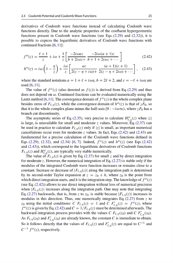
where the standard notations a = 1 + + iωη, b = 2 + 2, and c = − + iωη are
used [6, 11].
The value of f ω (z) (also denoted as f (z)) is derived from Eq. (2.29) and thus
does not depend on ω. Continued fractions can be evaluated numerically using the
Lentz method [6,11]. The convergence domain of f ω (z) is the whole complex plane
besides zeros of F ,η (z), while the convergence domain of h ω (z) is that of 2 F 0 , so
that it is the whole complex plane minus the half-axis [0 : −iω∞), where 2 F 0 has a
branch cut discontinuity.
The asymptotic series of Eq. (2.35), very precise to calculate H ω
,η (z) when |z|
is large, is unavailable for small and moderate z values. Moreover, Eq. (2.37) can
be used in practice to calculate F ,η (z) only if |z| is small, as important numerical
cancellations occur even for moderate z values. In fact, Eqs. (2.42) and (2.43) are
fundamental for a precise calculation of the Coulomb wave functions defined in
Eqs. (2.29), (2.32), and (2.34) [6, 7]. Indeed, f ω (z) and h ω (z) (see Eqs. (2.42)
and (2.43)), which correspond to the logarithmic derivatives of Coulomb functions
F ,η (z) and H ω
,η (z), are typically very stable numerically.
The value of F ,η (z) is given by Eq. (2.37) for small z and by direct integration
for moderate z. However, the numerical integration of Eq. (2.27) is stable only if the
modulus of the integrated Coulomb wave function increases or remains close to a
constant. Increase or decrease of |F ,η (z)| along the integration path is determined
by its second-order Taylor expansion at z = z 0 + h, where z 0 is the point from
which direct integration starts, and h is the integration step. The knowledge of f ω (z)
(see Eq. (2.42)) allows to use direct integration without loss of numerical precision
when |F ,η (z)| increases along the integration path. One may note that integrating
Eq. (2.27) backwards, that is, from z to z 0 , is stable because |F ,η (z)| increases in
modulus in this direction. Thus, one numerically integrates Eq. (2.27) from z to
z 0 using the initial conditions: C F ,η (z) = 1 and C F
,η (z) = f ω (z), where
f ω (z) is given by Eq. (2.42) and C = 1/F ,η (z) must be determined afterwards. The
backward integration process provides with the values C F ,η (z 0 ) and C F
,η (z 0 ).
As F ,η (z 0 ) and F
,η (z 0 ) are already known, the constant C is immediate to obtain.
So it follows directly that the values of F ,η (z) and F
,η (z) are equal to C −1 and
C −1 f ω (z), respectively.
25
derivatives of Coulomb wave functions instead of calculating Coulomb wave
functions directly. Due to the analytic properties of the confluent hypergeometric
functions present in Coulomb wave functions (see Eqs. (2.29) and (2.32)), it is
possible to express the logarithmic derivatives of Coulomb wave functions with
continued fractions [6, 11]:
f
ω (z) =
+ 1
z
+ iω +
1
z
−2iωaz
b + 2iωz+
−2iω(a + 1)z
b + 1 + 2iωz + · · ·
(2.42)
h
ω (z) = iω
1 −
η
z
+
iω
z
ac
2(z − η + iω)+
(a + 1)(c + 1)
2(z − η + 2iω) + · · ·
, (2.43)
where the standard notations a = 1 + + iωη, b = 2 + 2, and c = − + iωη are
used [6, 11].
The value of f ω (z) (also denoted as f (z)) is derived from Eq. (2.29) and thus
does not depend on ω. Continued fractions can be evaluated numerically using the
Lentz method [6,11]. The convergence domain of f ω (z) is the whole complex plane
besides zeros of F ,η (z), while the convergence domain of h ω (z) is that of 2 F 0 , so
that it is the whole complex plane minus the half-axis [0 : −iω∞), where 2 F 0 has a
branch cut discontinuity.
The asymptotic series of Eq. (2.35), very precise to calculate H ω
,η (z) when |z|
is large, is unavailable for small and moderate z values. Moreover, Eq. (2.37) can
be used in practice to calculate F ,η (z) only if |z| is small, as important numerical
cancellations occur even for moderate z values. In fact, Eqs. (2.42) and (2.43) are
fundamental for a precise calculation of the Coulomb wave functions defined in
Eqs. (2.29), (2.32), and (2.34) [6, 7]. Indeed, f ω (z) and h ω (z) (see Eqs. (2.42)
and (2.43)), which correspond to the logarithmic derivatives of Coulomb functions
F ,η (z) and H ω
,η (z), are typically very stable numerically.
The value of F ,η (z) is given by Eq. (2.37) for small z and by direct integration
for moderate z. However, the numerical integration of Eq. (2.27) is stable only if the
modulus of the integrated Coulomb wave function increases or remains close to a
constant. Increase or decrease of |F ,η (z)| along the integration path is determined
by its second-order Taylor expansion at z = z 0 + h, where z 0 is the point from
which direct integration starts, and h is the integration step. The knowledge of f ω (z)
(see Eq. (2.42)) allows to use direct integration without loss of numerical precision
when |F ,η (z)| increases along the integration path. One may note that integrating
Eq. (2.27) backwards, that is, from z to z 0 , is stable because |F ,η (z)| increases in
modulus in this direction. Thus, one numerically integrates Eq. (2.27) from z to
z 0 using the initial conditions: C F ,η (z) = 1 and C F
,η (z) = f ω (z), where
f ω (z) is given by Eq. (2.42) and C = 1/F ,η (z) must be determined afterwards. The
backward integration process provides with the values C F ,η (z 0 ) and C F
,η (z 0 ).
As F ,η (z 0 ) and F
,η (z 0 ) are already known, the constant C is immediate to obtain.
So it follows directly that the values of F ,η (z) and F
,η (z) are equal to C −1 and
C −1 f ω (z), respectively.