

2.3 Coulomb Potential and Coulomb Wave Functions
23
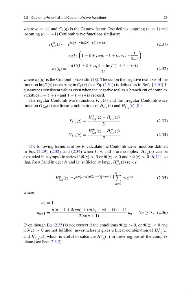
where ω = ±1 and C (η) is the Gamow factor. One defines outgoing (ω = 1) and
incoming (ω = −1) Coulomb wave functions similarly:
H
ω
,η (z) = e
iω[z−η ln(2z)−
π
2 +σ (η)]
(2.31)
× 2 F 0
1 + + iωη, − + iωη; ; −
i
2ωz
σ (η) =
ln(Γ (1 + + iη)) − ln(Γ (1 + − iη))
2i
,
(2.32)
where σ (η) is the Coulomb phase shift [8]. The cut on the negative real axis of the
function ln(Γ (z)) occurring in C (η) (see Eq. (2.31)) is defined as in Refs. [9,10]. It
guarantees consistent values even when the negative real axis branch cut of complex
variables 1 + + iη and 1 + − iη is crossed.
The regular Coulomb wave function F ,η (z) and the irregular Coulomb wave
function G ,η (z) are linear combinations of H
+
,η (z) and H
−
,η (z) [8]:
F ,η (z) =
H
+
,η (z) − H
−
,η (z)
2i
(2.33)
G ,η (z) =
H
+
,η (z) + H
−
,η (z)
2
.
(2.34)
The following formulas allow to calculate the Coulomb wave functions defined
in Eqs. (2.29), (2.32), and (2.34) when η, and z are complex. H ω
,η (z) can be
expanded in asymptotic series if (z) > 0 or (z) < 0 and ω(z) > 0 [6, 11], so
that, for a fixed integer N and |z| sufficiently large, H ω
,η (z) reads:
H
ω
,η (z) e
iω[z−η ln(2z)−
π
2 +σ (η)]
N−1
n=0
a n z
−n ,
(2.35)
where
a 0 = 1
a n+1 =
n(n + 1 + 2iωη) + iη(iη + ω) − + 1)
2iω(n + 1)
a n
∀n ≥ 0 . (2.36)
Even though Eq. (2.35) is not correct if the conditions (z) > 0, or (z) < 0 and
ω(z) > 0 are not fulfilled, nevertheless it gives a linear combination of H
+
,η (z)
and H
−
,η (z), which is useful to calculate H ω
,η (z) in these regions of the complex
plane (see Sect. 2.3.2).
23
where ω = ±1 and C (η) is the Gamow factor. One defines outgoing (ω = 1) and
incoming (ω = −1) Coulomb wave functions similarly:
H
ω
,η (z) = e
iω[z−η ln(2z)−
π
2 +σ (η)]
(2.31)
× 2 F 0
1 + + iωη, − + iωη; ; −
i
2ωz
σ (η) =
ln(Γ (1 + + iη)) − ln(Γ (1 + − iη))
2i
,
(2.32)
where σ (η) is the Coulomb phase shift [8]. The cut on the negative real axis of the
function ln(Γ (z)) occurring in C (η) (see Eq. (2.31)) is defined as in Refs. [9,10]. It
guarantees consistent values even when the negative real axis branch cut of complex
variables 1 + + iη and 1 + − iη is crossed.
The regular Coulomb wave function F ,η (z) and the irregular Coulomb wave
function G ,η (z) are linear combinations of H
+
,η (z) and H
−
,η (z) [8]:
F ,η (z) =
H
+
,η (z) − H
−
,η (z)
2i
(2.33)
G ,η (z) =
H
+
,η (z) + H
−
,η (z)
2
.
(2.34)
The following formulas allow to calculate the Coulomb wave functions defined
in Eqs. (2.29), (2.32), and (2.34) when η, and z are complex. H ω
,η (z) can be
expanded in asymptotic series if (z) > 0 or (z) < 0 and ω(z) > 0 [6, 11], so
that, for a fixed integer N and |z| sufficiently large, H ω
,η (z) reads:
H
ω
,η (z) e
iω[z−η ln(2z)−
π
2 +σ (η)]
N−1
n=0
a n z
−n ,
(2.35)
where
a 0 = 1
a n+1 =
n(n + 1 + 2iωη) + iη(iη + ω) − + 1)
2iω(n + 1)
a n
∀n ≥ 0 . (2.36)
Even though Eq. (2.35) is not correct if the conditions (z) > 0, or (z) < 0 and
ω(z) > 0 are not fulfilled, nevertheless it gives a linear combination of H
+
,η (z)
and H
−
,η (z), which is useful to calculate H ω
,η (z) in these regions of the complex
plane (see Sect. 2.3.2).