

5.6 Calculation of Two-Body Matrix Elements in the Gamow Shell Model
213
calculation of its matrix elements is equivalent to calculating the Fourier-Bessel
transform of r 2 , which is proportional to δ (k − k ). A direct numerical treatment
of derivatives of the Dirac delta would be cumbersome as one would have to
differentiate numerically the scattering components of the Gamow shell model
eigenvector with respect to k. Conversely, Eq. (5.66) provides with well-defined
matrix elements of electromagnetic operators. Moreover, it has been checked
numerically that convergence with the number of used harmonic oscillator shells is
rather fast in loosely bound or narrow resonance many-body states. Consequently,
the harmonic oscillator expansion of Eq. (5.66) is the method of choice to deal with
observables whose radial operator increases on the real axis.
This method is applied to the 6 He and 18 O nuclei, modeled by two neutrons
above a core. One uses 4 He core for 6 He and 16 O core for 18 O. The N 3 LO realistic
interaction renormalized with the V low-k method [27] is used for nucleon-nucleon
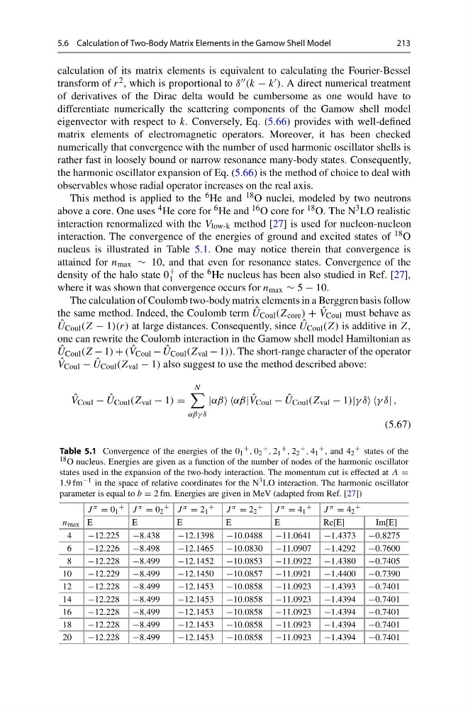
interaction. The convergence of the energies of ground and excited states of 18 O
nucleus is illustrated in Table 5.1. One may notice therein that convergence is
attained for n max ∼ 10, and that even for resonance states. Convergence of the
density of the halo state 0
+
1 of the 6 He nucleus has been also studied in Ref. [27],
where it was shown that convergence occurs for n max ∼ 5 − 10.
The calculation of Coulomb two-body matrix elements in a Berggren basis follow
the same method. Indeed, the Coulomb term ˆ
U Coul (Z core ) + ˆ
V Coul must behave as
ˆ
U Coul (Z − 1)(r) at large distances. Consequently, since ˆ
U Coul (Z) is additive in Z,
one can rewrite the Coulomb interaction in the Gamow shell model Hamiltonian as
ˆ
U Coul (Z − 1) + ( ˆ
V Coul − ˆ
U Coul (Z val − 1)). The short-range character of the operator
ˆ
V Coul − ˆ
U Coul (Z val − 1) also suggest to use the method described above:
ˆ
V Coul − ˆ
U Coul (Z val − 1) =
N
αβγ δ
|αβ αβ| ˆ
V Coul − ˆ
U Coul (Z val − 1)|γ δ γ δ| ,
(5.67)
Table 5.1 Convergence of the energies of the 0 1
+ , 0 2
+ , 2 1
+ , 2 2
+ , 4 1
+ , and 4 2
+ states of the
18 O nucleus. Energies are given as a function of the number of nodes of the harmonic oscillator
states used in the expansion of the two-body interaction. The momentum cut is effected at Λ =
1.9 fm
−1 in the space of relative coordinates for the N 3 LO interaction. The harmonic oscillator
parameter is equal to b = 2 fm. Energies are given in MeV (adapted from Ref. [27])
J π = 0 1
+ J π = 0 2
+ J π = 2 1
+
J π = 2 2
+
J π = 4 1
+
J π = 4 2
+
n max E
E
E
E
E
Re[E]
Im[E]
4
−12.225 −8.438
−12.1398 −10.0488 −11.0641 −1.4373 −0.8275
6
−12.226 −8.498
−12.1465 −10.0830 −11.0907 −1.4292 −0.7600
8
−12.228 −8.499
−12.1452 −10.0853 −11.0922 −1.4380 −0.7405
10
−12.229 −8.499
−12.1450 −10.0857 −11.0921 −1.4400 −0.7390
12
−12.228 −8.499
−12.1453 −10.0858 −11.0923 −1.4393 −0.7401
14
−12.228 −8.499
−12.1453 −10.0858 −11.0923 −1.4394 −0.7401
16
−12.228 −8.499
−12.1453 −10.0858 −11.0923 −1.4394 −0.7401
18
−12.228 −8.499
−12.1453 −10.0858 −11.0923 −1.4394 −0.7401
20
−12.228 −8.499
−12.1453 −10.0858 −11.0923 −1.4394 −0.7401
213
calculation of its matrix elements is equivalent to calculating the Fourier-Bessel
transform of r 2 , which is proportional to δ (k − k ). A direct numerical treatment
of derivatives of the Dirac delta would be cumbersome as one would have to
differentiate numerically the scattering components of the Gamow shell model
eigenvector with respect to k. Conversely, Eq. (5.66) provides with well-defined
matrix elements of electromagnetic operators. Moreover, it has been checked
numerically that convergence with the number of used harmonic oscillator shells is
rather fast in loosely bound or narrow resonance many-body states. Consequently,
the harmonic oscillator expansion of Eq. (5.66) is the method of choice to deal with
observables whose radial operator increases on the real axis.
This method is applied to the 6 He and 18 O nuclei, modeled by two neutrons
above a core. One uses 4 He core for 6 He and 16 O core for 18 O. The N 3 LO realistic
interaction renormalized with the V low-k method [27] is used for nucleon-nucleon
interaction. The convergence of the energies of ground and excited states of 18 O
nucleus is illustrated in Table 5.1. One may notice therein that convergence is
attained for n max ∼ 10, and that even for resonance states. Convergence of the
density of the halo state 0
+
1 of the 6 He nucleus has been also studied in Ref. [27],
where it was shown that convergence occurs for n max ∼ 5 − 10.
The calculation of Coulomb two-body matrix elements in a Berggren basis follow
the same method. Indeed, the Coulomb term ˆ
U Coul (Z core ) + ˆ
V Coul must behave as
ˆ
U Coul (Z − 1)(r) at large distances. Consequently, since ˆ
U Coul (Z) is additive in Z,
one can rewrite the Coulomb interaction in the Gamow shell model Hamiltonian as
ˆ
U Coul (Z − 1) + ( ˆ
V Coul − ˆ
U Coul (Z val − 1)). The short-range character of the operator
ˆ
V Coul − ˆ
U Coul (Z val − 1) also suggest to use the method described above:
ˆ
V Coul − ˆ
U Coul (Z val − 1) =
N
αβγ δ
|αβ αβ| ˆ
V Coul − ˆ
U Coul (Z val − 1)|γ δ γ δ| ,
(5.67)
Table 5.1 Convergence of the energies of the 0 1
+ , 0 2
+ , 2 1
+ , 2 2
+ , 4 1
+ , and 4 2
+ states of the
18 O nucleus. Energies are given as a function of the number of nodes of the harmonic oscillator
states used in the expansion of the two-body interaction. The momentum cut is effected at Λ =
1.9 fm
−1 in the space of relative coordinates for the N 3 LO interaction. The harmonic oscillator
parameter is equal to b = 2 fm. Energies are given in MeV (adapted from Ref. [27])
J π = 0 1
+ J π = 0 2
+ J π = 2 1
+
J π = 2 2
+
J π = 4 1
+
J π = 4 2
+
n max E
E
E
E
E
Re[E]
Im[E]
4
−12.225 −8.438
−12.1398 −10.0488 −11.0641 −1.4373 −0.8275
6
−12.226 −8.498
−12.1465 −10.0830 −11.0907 −1.4292 −0.7600
8
−12.228 −8.499
−12.1452 −10.0853 −11.0922 −1.4380 −0.7405
10
−12.229 −8.499
−12.1450 −10.0857 −11.0921 −1.4400 −0.7390
12
−12.228 −8.499
−12.1453 −10.0858 −11.0923 −1.4393 −0.7401
14
−12.228 −8.499
−12.1453 −10.0858 −11.0923 −1.4394 −0.7401
16
−12.228 −8.499
−12.1453 −10.0858 −11.0923 −1.4394 −0.7401
18
−12.228 −8.499
−12.1453 −10.0858 −11.0923 −1.4394 −0.7401
20
−12.228 −8.499
−12.1453 −10.0858 −11.0923 −1.4394 −0.7401