

142
3 Berggren Basis and Completeness Relations
Exercise XI.
A. Radial integrals always converge with complex scaling when k = k (see
Sect. 3.3). On the other hand, it is more complicated to calculate radial integrals
for which k = k and ω a ω b = −1 with complex rotation (see Sect. 3.4). To show
that these integrals converge, one considers k ∼ k as
c k − c k ∼
(k − k) n
n!
∂ n c κ
∂κ n
κ=k
,
where n ≥ 1 is the smallest integer so that the partial derivative is not equal to
zero, as c k is an analytic function of k. The asymptote of u
±
k (r) for r → +∞ is
provided by Eq. (2.7) and one uses 2π C + C − = 1 (see Eq. (3.19)).
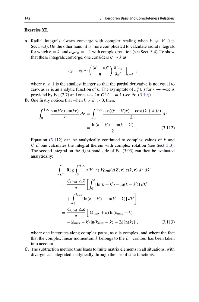
B. One firstly notices that when k > k > 0, then:
+∞
0
sin(k r) sin(kr)
r
dr =
+∞
0
cos((k − k )r) − cos((k + k )r)
2r
dr
=
ln(k + k ) − ln(k − k )
2
.
(3.112)
Equation (3.112) can be analytically continued to complex values of k and
k if one calculates the integral therein with complex rotation (see Sect. 3.3).
The second integral on the right-hand side of Eq. (3.93) can then be evaluated
analytically:
L +
Reg
+∞
0
s(k
, r) V Coul (ΔZ, r) s(k, r) dr dk
=
C Coul ΔZ
π
k
0
[ln(k + k
) − ln(k − k
)] dk
+
k max
k
[ln(k + k
) − ln(k
− k)] dk
=
C Coul ΔZ
π
(k max + k) ln(k max + k)
−(k max − k) ln(k max − k) − 2k ln(k)] ,
(3.113)
where one integrates along complex paths, as k is complex, and where the fact
that the complex linear momentum k belongs to the L + contour has been taken
into account.
C. The subtraction method thus leads to finite matrix elements in all situations, with
divergences integrated analytically through the use of sine functions.
3 Berggren Basis and Completeness Relations
Exercise XI.
A. Radial integrals always converge with complex scaling when k = k (see
Sect. 3.3). On the other hand, it is more complicated to calculate radial integrals
for which k = k and ω a ω b = −1 with complex rotation (see Sect. 3.4). To show
that these integrals converge, one considers k ∼ k as
c k − c k ∼
(k − k) n
n!
∂ n c κ
∂κ n
κ=k
,
where n ≥ 1 is the smallest integer so that the partial derivative is not equal to
zero, as c k is an analytic function of k. The asymptote of u
±
k (r) for r → +∞ is
provided by Eq. (2.7) and one uses 2π C + C − = 1 (see Eq. (3.19)).
B. One firstly notices that when k > k > 0, then:
+∞
0
sin(k r) sin(kr)
r
dr =
+∞
0
cos((k − k )r) − cos((k + k )r)
2r
dr
=
ln(k + k ) − ln(k − k )
2
.
(3.112)
Equation (3.112) can be analytically continued to complex values of k and
k if one calculates the integral therein with complex rotation (see Sect. 3.3).
The second integral on the right-hand side of Eq. (3.93) can then be evaluated
analytically:
L +
Reg
+∞
0
s(k
, r) V Coul (ΔZ, r) s(k, r) dr dk
=
C Coul ΔZ
π
k
0
[ln(k + k
) − ln(k − k
)] dk
+
k max
k
[ln(k + k
) − ln(k
− k)] dk
=
C Coul ΔZ
π
(k max + k) ln(k max + k)
−(k max − k) ln(k max − k) − 2k ln(k)] ,
(3.113)
where one integrates along complex paths, as k is complex, and where the fact
that the complex linear momentum k belongs to the L + contour has been taken
into account.
C. The subtraction method thus leads to finite matrix elements in all situations, with
divergences integrated analytically through the use of sine functions.