

134
3 Berggren Basis and Completeness Relations
10
-1
Time (s)
Matrix dimension
0 100 200 300 400 500 600 700 800 900 1000
10
-2
10
0
10
1
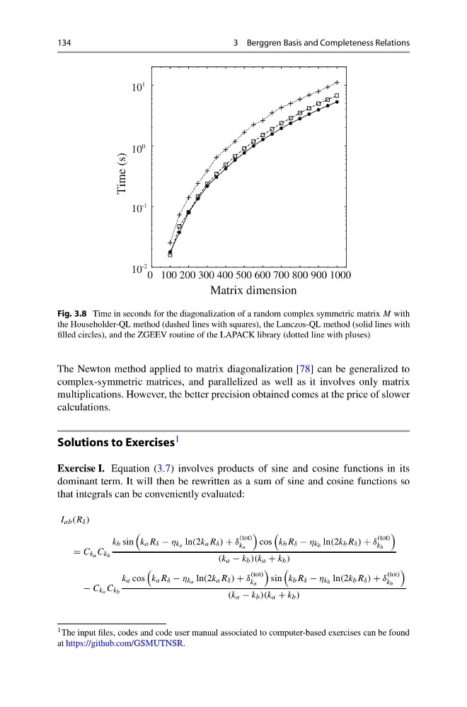
Fig. 3.8 Time in seconds for the diagonalization of a random complex symmetric matrix M with
the Householder-QL method (dashed lines with squares), the Lanczos-QL method (solid lines with
filled circles), and the ZGEEV routine of the LAPACK library (dotted line with pluses)
The Newton method applied to matrix diagonalization [78] can be generalized to
complex-symmetric matrices, and parallelized as well as it involves only matrix
multiplications. However, the better precision obtained comes at the price of slower
calculations.
Solutions to Exercises 1
Exercise I. Equation (3.7) involves products of sine and cosine functions in its
dominant term. It will then be rewritten as a sum of sine and cosine functions so
that integrals can be conveniently evaluated:
I ab (R δ )
= C ka C k b
k b sin
k a R δ − η ka ln(2k a R δ ) + δ
(tot)
ka
cos
k b R δ − η k b ln(2k b R δ ) + δ
(tot)
k b
(k a − k b )(k a + k b )
− C ka C k b
k a cos
k a R δ − η ka ln(2k a R δ ) + δ
(tot)
ka
sin
k b R δ − η k b ln(2k b R δ ) + δ
(tot)
k b
(k a − k b )(k a + k b )
1 The input files, codes and code user manual associated to computer-based exercises can be found
at https://github.com/GSMUTNSR.
3 Berggren Basis and Completeness Relations
10
-1
Time (s)
Matrix dimension
0 100 200 300 400 500 600 700 800 900 1000
10
-2
10
0
10
1
Fig. 3.8 Time in seconds for the diagonalization of a random complex symmetric matrix M with
the Householder-QL method (dashed lines with squares), the Lanczos-QL method (solid lines with
filled circles), and the ZGEEV routine of the LAPACK library (dotted line with pluses)
The Newton method applied to matrix diagonalization [78] can be generalized to
complex-symmetric matrices, and parallelized as well as it involves only matrix
multiplications. However, the better precision obtained comes at the price of slower
calculations.
Solutions to Exercises 1
Exercise I. Equation (3.7) involves products of sine and cosine functions in its
dominant term. It will then be rewritten as a sum of sine and cosine functions so
that integrals can be conveniently evaluated:
I ab (R δ )
= C ka C k b
k b sin
k a R δ − η ka ln(2k a R δ ) + δ
(tot)
ka
cos
k b R δ − η k b ln(2k b R δ ) + δ
(tot)
k b
(k a − k b )(k a + k b )
− C ka C k b
k a cos
k a R δ − η ka ln(2k a R δ ) + δ
(tot)
ka
sin
k b R δ − η k b ln(2k b R δ ) + δ
(tot)
k b
(k a − k b )(k a + k b )
1 The input files, codes and code user manual associated to computer-based exercises can be found
at https://github.com/GSMUTNSR.