

3.7 Numerical Implementation of the Berggren Completeness Relation
115
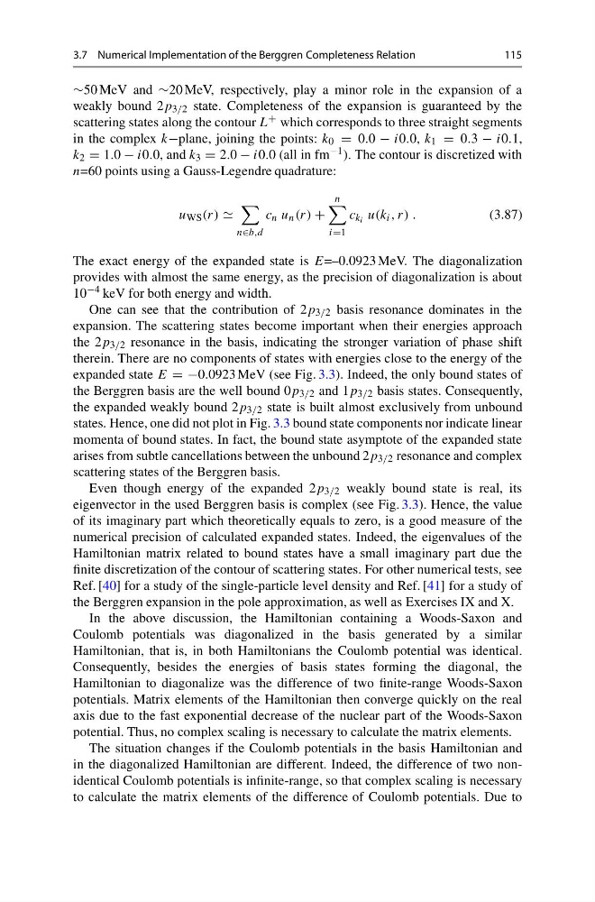
∼50 MeV and ∼20 MeV, respectively, play a minor role in the expansion of a
weakly bound 2p 3/2 state. Completeness of the expansion is guaranteed by the
scattering states along the contour L + which corresponds to three straight segments
in the complex k−plane, joining the points: k 0 = 0.0 − i0.0, k 1 = 0.3 − i0.1,
k 2 = 1.0 − i0.0, and k 3 = 2.0 − i0.0 (all in fm −1 ). The contour is discretized with
n=60 points using a Gauss-Legendre quadrature:
u WS (r)
n∈b,d
c n u n (r) +
n
i=1
c k i u(k i , r) .
(3.87)
The exact energy of the expanded state is E=–0.0923 MeV. The diagonalization
provides with almost the same energy, as the precision of diagonalization is about
10 −4 keV for both energy and width.
One can see that the contribution of 2p 3/2 basis resonance dominates in the
expansion. The scattering states become important when their energies approach
the 2p 3/2 resonance in the basis, indicating the stronger variation of phase shift
therein. There are no components of states with energies close to the energy of the
expanded state E = −0.0923 MeV (see Fig. 3.3). Indeed, the only bound states of
the Berggren basis are the well bound 0p 3/2 and 1p 3/2 basis states. Consequently,
the expanded weakly bound 2p 3/2 state is built almost exclusively from unbound
states. Hence, one did not plot in Fig. 3.3 bound state components nor indicate linear
momenta of bound states. In fact, the bound state asymptote of the expanded state
arises from subtle cancellations between the unbound 2p 3/2 resonance and complex
scattering states of the Berggren basis.
Even though energy of the expanded 2p 3/2 weakly bound state is real, its
eigenvector in the used Berggren basis is complex (see Fig. 3.3). Hence, the value
of its imaginary part which theoretically equals to zero, is a good measure of the
numerical precision of calculated expanded states. Indeed, the eigenvalues of the
Hamiltonian matrix related to bound states have a small imaginary part due the
finite discretization of the contour of scattering states. For other numerical tests, see
Ref. [40] for a study of the single-particle level density and Ref. [41] for a study of
the Berggren expansion in the pole approximation, as well as Exercises IX and X.
In the above discussion, the Hamiltonian containing a Woods-Saxon and
Coulomb potentials was diagonalized in the basis generated by a similar
Hamiltonian, that is, in both Hamiltonians the Coulomb potential was identical.
Consequently, besides the energies of basis states forming the diagonal, the
Hamiltonian to diagonalize was the difference of two finite-range Woods-Saxon
potentials. Matrix elements of the Hamiltonian then converge quickly on the real
axis due to the fast exponential decrease of the nuclear part of the Woods-Saxon
potential. Thus, no complex scaling is necessary to calculate the matrix elements.
The situation changes if the Coulomb potentials in the basis Hamiltonian and
in the diagonalized Hamiltonian are different. Indeed, the difference of two nonidentical Coulomb potentials is infinite-range, so that complex scaling is necessary
to calculate the matrix elements of the difference of Coulomb potentials. Due to
115
∼50 MeV and ∼20 MeV, respectively, play a minor role in the expansion of a
weakly bound 2p 3/2 state. Completeness of the expansion is guaranteed by the
scattering states along the contour L + which corresponds to three straight segments
in the complex k−plane, joining the points: k 0 = 0.0 − i0.0, k 1 = 0.3 − i0.1,
k 2 = 1.0 − i0.0, and k 3 = 2.0 − i0.0 (all in fm −1 ). The contour is discretized with
n=60 points using a Gauss-Legendre quadrature:
u WS (r)
n∈b,d
c n u n (r) +
n
i=1
c k i u(k i , r) .
(3.87)
The exact energy of the expanded state is E=–0.0923 MeV. The diagonalization
provides with almost the same energy, as the precision of diagonalization is about
10 −4 keV for both energy and width.
One can see that the contribution of 2p 3/2 basis resonance dominates in the
expansion. The scattering states become important when their energies approach
the 2p 3/2 resonance in the basis, indicating the stronger variation of phase shift
therein. There are no components of states with energies close to the energy of the
expanded state E = −0.0923 MeV (see Fig. 3.3). Indeed, the only bound states of
the Berggren basis are the well bound 0p 3/2 and 1p 3/2 basis states. Consequently,
the expanded weakly bound 2p 3/2 state is built almost exclusively from unbound
states. Hence, one did not plot in Fig. 3.3 bound state components nor indicate linear
momenta of bound states. In fact, the bound state asymptote of the expanded state
arises from subtle cancellations between the unbound 2p 3/2 resonance and complex
scattering states of the Berggren basis.
Even though energy of the expanded 2p 3/2 weakly bound state is real, its
eigenvector in the used Berggren basis is complex (see Fig. 3.3). Hence, the value
of its imaginary part which theoretically equals to zero, is a good measure of the
numerical precision of calculated expanded states. Indeed, the eigenvalues of the
Hamiltonian matrix related to bound states have a small imaginary part due the
finite discretization of the contour of scattering states. For other numerical tests, see
Ref. [40] for a study of the single-particle level density and Ref. [41] for a study of
the Berggren expansion in the pole approximation, as well as Exercises IX and X.
In the above discussion, the Hamiltonian containing a Woods-Saxon and
Coulomb potentials was diagonalized in the basis generated by a similar
Hamiltonian, that is, in both Hamiltonians the Coulomb potential was identical.
Consequently, besides the energies of basis states forming the diagonal, the
Hamiltonian to diagonalize was the difference of two finite-range Woods-Saxon
potentials. Matrix elements of the Hamiltonian then converge quickly on the real
axis due to the fast exponential decrease of the nuclear part of the Woods-Saxon
potential. Thus, no complex scaling is necessary to calculate the matrix elements.
The situation changes if the Coulomb potentials in the basis Hamiltonian and
in the diagonalized Hamiltonian are different. Indeed, the difference of two nonidentical Coulomb potentials is infinite-range, so that complex scaling is necessary
to calculate the matrix elements of the difference of Coulomb potentials. Due to